Lecture 11: Spark Dataframes#
Learning Objectives#
By the end of this lecture, students should be able to:
Understand the concept of Resilient Distributed Datasets (RDDs) in Apache Spark.
Explain the immutability and fault tolerance features of RDDs.
Describe how RDDs enable parallel processing in a distributed computing environment.
Identify the key features of RDDs, including lazy evaluation and partitioning.
Introducing Spark DataFrames#
Like an RDD, a DataFrame is an immutable distributed collection of data. Unlike an RDD, data is organized into named columns, like a table in a relational database. Designed to make large data sets processing even easier
Spark DataFrames are a distributed collection of data organized into named columns, similar to a table in a relational database. They provide a higher-level abstraction than RDDs, making it easier to work with structured and semi-structured data. DataFrames support a wide range of operations, including filtering, aggregation, and joining, and they are optimized for performance through the Catalyst query optimizer. This makes them a powerful tool for big data processing and analytics.
What makes a Spark DataFrame different from other dataframes such as pandas DataFrame is the distributed aspect of it, similar to the RDDs concept that we learned in the last lecture.
Suppose you have the following table stored in a Spark DataFrame:
ID |
Name |
Age |
City |
|---|---|---|---|
1 |
Alice |
30 |
New York |
2 |
Bob |
25 |
Los Angeles |
3 |
Charlie |
35 |
Chicago |
4 |
David |
40 |
Houston |
As a programmer, you will see, manage, and transform this table as if it was a single and unified table. However, under the hoods, Spark splits the data into multiple partitions across clusters.
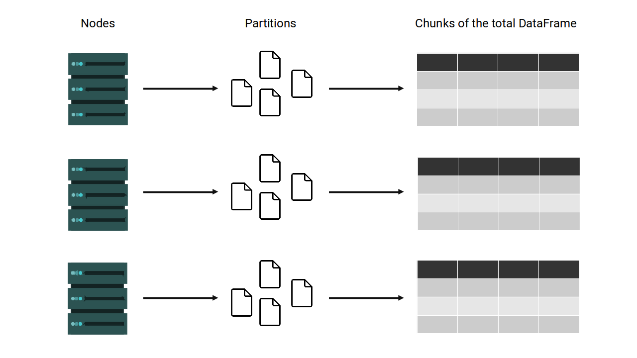
For the most part, you don’t manipulate these partitions manually or individually but instead rely on Spark’s built-in operations to handle the distribution and parallelism for you.
Create a DataFrame in pyspark#
Let’s create a sample spark dataframe
data = [("Alice", 34), ("Bob", 45), ("Cathy", 29)]
columns = ["Name", "Age"]

df = spark.createDataFrame(data, columns)
df
DataFrame[Name: string, Age: bigint]
Remember that a Spark DataFrame in python is a object of class pyspark.sql.dataframe.DataFrame as you can see below:
type(df)
pyspark.sql.dataframe.DataFrame
Let’s try to see what’s inside of df
df
DataFrame[Name: string, Age: bigint]
When we call for an object that stores a Spark DataFrame, Spark will only calculate and print a summary of the structure of your Spark DataFrame, and not the DataFrame itself.
To actually see the Spark DataFrame, you need to use the show() method.
df.show(2)
+-----+---+
| Name|Age|
+-----+---+
|Alice| 34|
|  Bob| 45|
+-----+---+
only showing top 2 rows
You can also show top n rows by using show(n)
df.show(2)
+-----+---+
| Name|Age|
+-----+---+
|Alice| 34|
|  Bob| 45|
+-----+---+
only showing top 2 rows
You could also display top n rows using the take() function, but the output is a list of Row objects, not formatted as a table.
df.take(2)
[Row(Name='Alice', Age=34), Row(Name='Bob', Age=45)]
Let’s get the name of the columns
df.columns
['Name', 'Age']
Let’s get the number of rows
df.count()
3
Data types and schema in Spark DataFrames#
The schema of a Spark DataFrame is the combination of column names and the data types associated with each of these columns
df.printSchema()
root
 |-- Name: string (nullable = true)
 |-- Age: long (nullable = true)
When Spark creates a new DataFrame, it will automatically guess which schema is appropriate for that DataFrame. In other words, Spark will try to guess which are the appropriate data types for each column.
You can create a dataframe with a predefined schema. For example, we want to set Age as integer
from pyspark.sql.types import StructType, StructField, StringType, IntegerType
from pyspark.sql import Row

schema = StructType([
    StructField("Name", StringType(), True),
    StructField("Age", IntegerType(), True)
])

data = [Row(Name="Alice", Age=30), Row(Name="Bob", Age=25), Row(Name="Charlie", Age=35)]

sample_df = spark.createDataFrame(data, schema)
sample_df.printSchema()
root
 |-- Name: string (nullable = true)
 |-- Age: integer (nullable = true)
Besides the “standard” data types such as Integer, Float, Double, String, etc…, Spark DataFrame also support two more complex types which are ArrayType and MapType:
ArrayType represents a column that contains an array of elements.
from pyspark.sql.types import StructType, StructField, StringType, ArrayType

# Define schema with ArrayType
schema = StructType([
    StructField("Name", StringType(), True),
    StructField("Hobbies", ArrayType(StringType()), True)
])

# Sample data
data = [
    ("Alice", ["Reading", "Hiking"]),
    ("Bob", ["Cooking", "Swimming"]),
    ("Cathy", ["Traveling", "Dancing"])
]

# Create DataFrame
df = spark.createDataFrame(data, schema)
df.show()
+-----+--------------------+
| Name|             Hobbies|
+-----+--------------------+
|Alice|   [Reading, Hiking]|
|  Bob| [Cooking, Swimming]|
|Cathy|[Traveling, Dancing]|
+-----+--------------------+
MapType represents a column that contains a map of key-value pairs.
from pyspark.sql.types import StructType, StructField, StringType, MapType

# Define schema with MapType
schema = StructType([
    StructField("Name", StringType(), True),
    StructField("Attributes", MapType(StringType(), StringType()), True)
])

# Sample data
data = [
    ("Alice", {"Height": "5.5", "Weight": "130"}),
    ("Bob", {"Height": "6.0", "Weight": "180"}),
    ("Cathy", {"Height": "5.7", "Weight": "150"})
]

# Create DataFrame
df = spark.createDataFrame(data, schema)
df.show()
+-----+--------------------+
| Name|          Attributes|
+-----+--------------------+
|Alice|{Height -> 5.5, W...|
|  Bob|{Height -> 6.0, W...|
|Cathy|{Height -> 5.7, W...|
+-----+--------------------+
Transformations of Spark DataFrame#
List of Transformations in Spark DataFrame
select()filter()groupBy()agg()join()withColumn()drop()distinct()orderBy()limit()
data = [("Alice", 34), ("Bob", 45), ("Cathy", 29)]
columns = ["Name", "Age"]

df = spark.createDataFrame(data, columns)
df.select("Name").show()
+-----+
| Name|
+-----+
|Alice|
|  Bob|
|Cathy|
+-----+
df.filter(df.Name == 'Alice').show()
+-----+---+
| Name|Age|
+-----+---+
|Alice| 34|
+-----+---+
from pyspark.sql.functions import col
df.filter(col("Age") < 30).show()
+-----+---+
| Name|Age|
+-----+---+
|Cathy| 29|
+-----+---+
df2 = df\
    .filter(df.Age > 30)\
    .select("Name")
df2.show()
+-----+
| Name|
+-----+
|Alice|
|  Bob|
+-----+
Each one of these DataFrame methods create a lazily evaluated transformation. Spark will only check if they make sense with the initial DataFrame that you have. Spark will not actually perform these transformations on your initial DataFrame, not untill you trigger these transformations with an action.
df2.show()
+-----+
| Name|
+-----+
|Alice|
|  Bob|
+-----+
you can use a multi-line string to define a condition for filtering a DataFrame in PySpark
condition = '''
    Age < 30
    or Name = 'Alice'
'''
df.filter(condition).show()
+-----+---+
| Name|Age|
+-----+---+
|Alice| 34|
|Cathy| 29|
+-----+---+
Actions in Spark DataFrame#
Here are some common actions in Spark DataFrame, grouped by similarity:
Show and Display
show()head()first()take()
Aggregation and Statistics
count()describe()summary()agg()
Collection and Conversion
collect()toPandas()toJSON()
Saving and Writing
write()save()saveAsTable()
df.show()
+-----+---+
| Name|Age|
+-----+---+
|Alice| 34|
|  Bob| 45|
|Cathy| 29|
+-----+---+
df.sample(True, 0.5).show()
+-----+---+
| Name|Age|
+-----+---+
|  Bob| 45|
|Cathy| 29|
+-----+---+