Tutorial 3: PyTorch implementation on linear and logistic regression

Part 1: The “Black Box” vs. The “Glass Box”¶

Goal: Establish why we are learning a complex tool (PyTorch) for a simple problem (Linear Regression).

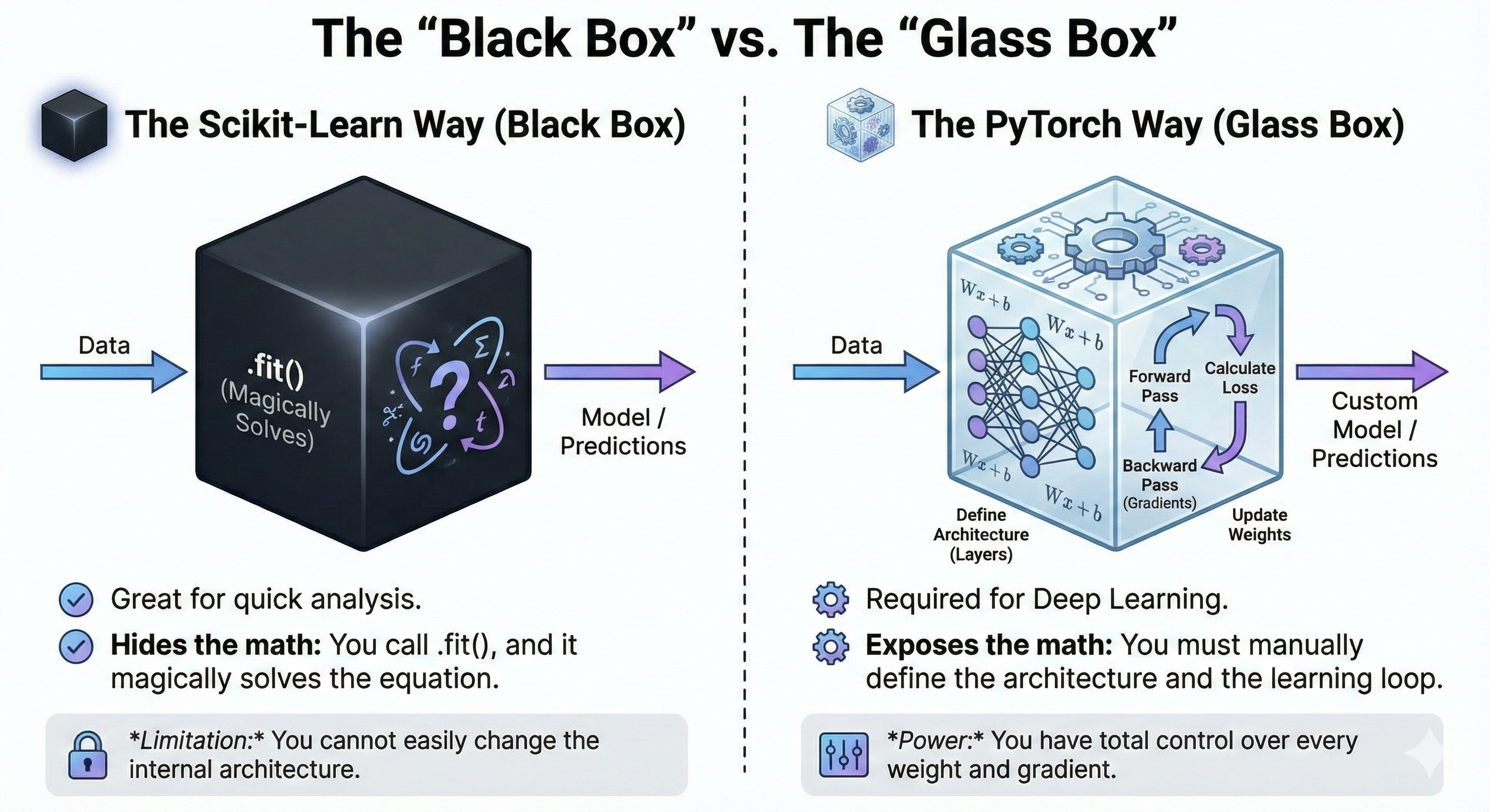
The Scikit-Learn Way (Black Box):

Great for quick analysis.
Hides the math: You call .fit(), and it magically solves the equation.
Limitation: You cannot easily change the internal architecture.

The PyTorch Way (Glass Box):

Required for Deep Learning.
Exposes the math: You must manually define the architecture and the learning loop.
Power: You have total control over every weight and gradient.

The scikit-learn way¶

import numpy as np
from sklearn.linear_model import LinearRegression

# Sample data
X = np.array([[1], [2], [3], [4]], dtype=np.float32)
y = np.array([[2], [4], [6], [8]], dtype=np.float32)

# Fit model
model = LinearRegression()
model.fit(X, y)

# Predict
pred = model.predict(X)
print("scikit-learn predictions:", pred.flatten())

scikit-learn predictions: [2. 4. 6. 8.]

The PyTorch way¶

import torch
import torch.nn as nn
import torch.optim as optim

# --- DATA ---
X = torch.tensor([[1.0], [2.0], [3.0], [4.0]])
y = torch.tensor([[2.0], [4.0], [6.0], [8.0]])

# --- STEP 1 & 2: The Model is a Class ---
class LinearRegressionOOP(nn.Module):
    def __init__(self):
        super().__init__()
        self.linear = nn.Linear(1, 1) 
    
    def forward(self, x):
        return self.linear(x) 

model = LinearRegressionOOP()

# --- STEP 3: The Loss & Optimizer 
criterion = nn.MSELoss()
optimizer = optim.SGD(model.parameters(), lr=0.01) 

# --- STEP 4: The Training Loop ---
for epoch in range(40):
    # 1. Forward
    pred = model(X)
    
    # 2. Loss
    loss = criterion(pred, y)
    
    # 3. Backward
    loss.backward()
    
    # 4. Update 
    optimizer.step()
    
    # 5. Zero Gradients
    optimizer.zero_grad()
    
    if epoch % 5 == 0:
        current_w = model.linear.weight.item()
        current_b = model.linear.bias.item()
        print(f"Epoch {epoch}: w={current_w:.3f}, b={current_b:.3f}, loss={loss.item():.3f}")

Epoch 0: w=0.671, b=-0.391, loss=23.056
Epoch 5: w=1.456, b=-0.125, loss=3.709
Epoch 10: w=1.771, b=-0.018, loss=0.597
Epoch 15: w=1.898, b=0.024, loss=0.096
Epoch 20: w=1.949, b=0.040, loss=0.016
Epoch 25: w=1.969, b=0.046, loss=0.003
Epoch 30: w=1.977, b=0.048, loss=0.001
Epoch 35: w=1.981, b=0.049, loss=0.000

Part 2: The Prerequisite – OOP for Deep Learning¶

Goal: Demystify the class structure students see in every PyTorch tutorial.

The Concept¶

Deep Learning models are complex software objects. We use Object-Oriented Programming (OOP) to organize them.

Class: The Blueprint (e.g., The schematic for a robot).
Object (Instance): The actual Robot built from the schematic.
self: The “Me” pointer. It allows the object to remember its own specific data.

The Analogy: The Robot Factory¶

class Robot:
    def __init__(self, name, color):
        # The Constructor: Runs automatically when created.
        # We attach data to 'self' so the robot remembers it.
        self.name = name
        self.color = color

    def introduce(self):
        # We access the saved data using 'self'
        return f"I am {self.name}, painted {self.color}."
    
    def help(self):
        return f"Hi, this is Costco. How can I help you"

robot2 = Robot("mehdi", "pink")

robot2.introduce()

'I am mehdi, painted pink.'

robot2.help()

'Hi, this is Costco. How can I help you'

robot3 = Robot("Varsha", "Light green")

robot3.introduce()

'I am Varsha, painted Light green.'

robot3.help()

'Hi, this is Costco. How can I help you'

r1 = Robot("Wall-E", "yellow")

print(r1.__dict__)

{'name': 'Wall-E', 'color': 'yellow'}

print(r1.name)

Wall-E

print(r1.color)

yellow

r1.introduce()

'I am Wall-E, painted yellow.'

Inheritance: BattleBot is a Robot, but with extra features¶

class BattleBot(Robot):
    def __init__(self, name, color, weapon):
        # SUPER: Call the parent class to handle basic setup (name/color)
        super().__init__(name, color) 
        self.weapon = weapon

    def attack(self):
        return f"{self.name} attacks with {self.weapon}!"

robot4 = BattleBot("Mint", "Red Brown", "Sword")

robot4.attack()

'Mint attacks with Sword!'

b1 = BattleBot("Terminator", "Red", "Machine guns")

print(b1.__dict__)

print(f"{b1.name}\n{b1.color}\n{b1.weapon}")

Terminator
Red
Machine guns

b1.attack()

'Terminator attacks with Machine guns!'

Connect to PyTorch:

BattleBot MyNeuralNetwork
Robot nn.Module (The parent class that gives us AI superpowers)
weapon self.layer1 (The specific layers we add)

Part 3: Implementation – The PyTorch OOP Way¶

Goal: Transition to the industry-standard workflow.

1. The Layer: `nn.Linear`¶

Explain that a “Layer” is just a container for the Weights () and Bias ().

Code: self.linear = nn.Linear(in_features=3, out_features=1)
Visual:
- Input (3): Square Footage, Rooms, Age.
- Output (1): Price.
- Internals: PyTorch creates a Weight Matrix and a size Bias Vector.

2. The Model Class¶

import torch
import torch.nn as nn
import torch.optim as optim

# --- DATA ---
X = torch.tensor([[1.0], [2.0], [3.0], [4.0]])
y = torch.tensor([[2.0], [4.0], [6.0], [8.0]])

# --- STEP 1 & 2: The Model is a Class ---
class LR_fun(nn.Module):
    def __init__(self):
        super().__init__()
        # nn.Linear automatically creates 'w' and 'b' for us inside this layer
        self.linear = nn.Linear(1, 1) 
    
    def forward(self, x):
        return self.linear(x) # Automatically does 'x @ w + b'
    
    def bark(self):
        return f"wofff"


model = LR_fun()

tensor([[1.],
        [2.],
        [3.],
        [4.]])

tensor([[2.],
        [4.],
        [6.],
        [8.]])

y_pred = model.forward(X)
y_pred

tensor([[-0.1714],
        [ 0.1175],
        [ 0.4064],
        [ 0.6953]], grad_fn=<AddmmBackward0>)

for param in model.parameters():
    print(param)

Parameter containing:
tensor([[0.2889]], requires_grad=True)
Parameter containing:
tensor([-0.4603], requires_grad=True)

3. The Training Loop¶

Walk through the 5 Steps that never change, whether it’s Linear Regression or ChatGPT.

Forward Pass: pred = model(x)
Calculate Loss: loss = criterion(pred, y)
Backward Pass: loss.backward() (Calculate gradients)
Optimizer Step: optimizer.step() (Update weights)
Zero Gradients: optimizer.zero_grad() (Clean up for next loop)


# --- STEP 3: The Loss & Optimizer are Classes ---
criterion = nn.MSELoss()

y_pred

tensor([[-0.1714],
        [ 0.1175],
        [ 0.4064],
        [ 0.6953]], grad_fn=<AddmmBackward0>)

tensor([[2.],
        [4.],
        [6.],
        [8.]])

criterion(y_pred,y)

tensor(26.1088, grad_fn=<MseLossBackward0>)

loss = criterion(y_pred, y)
    
    # 3. Backward
loss.backward()

optimizer = optim.SGD(model.parameters(), lr=0.01) # Handles the update step!

optimizer.step()

for param in model.parameters():
    print(param)

Parameter containing:
tensor([[0.5686]], requires_grad=True)
Parameter containing:
tensor([-0.3656], requires_grad=True)


# --- STEP 4: The Training Loop ---
for epoch in range(200):
    # 1. Forward
    pred = model(X)
    
    # 2. Loss
    loss = criterion(pred, y)
    
    # 3. Backward
    loss.backward()
    
    # 4. Update (Optimizer handles the 'no_grad' and math)
    optimizer.step()
    
    # 5. Zero Gradients
    optimizer.zero_grad()
    
    if epoch % 20 == 0:
        # Accessing weights requires digging into the object
        current_w = model.linear.weight.item()
        current_b = model.linear.bias.item()
        print(f"Epoch {epoch}: w={current_w:.3f}, b={current_b:.3f}, loss={loss.item():.3f}")

Epoch 0: w=1.924, b=0.222, loss=0.008
Epoch 20: w=1.929, b=0.210, loss=0.007
Epoch 40: w=1.933, b=0.197, loss=0.007
Epoch 60: w=1.937, b=0.186, loss=0.006
Epoch 80: w=1.940, b=0.175, loss=0.005
Epoch 100: w=1.944, b=0.165, loss=0.005
Epoch 120: w=1.947, b=0.155, loss=0.004
Epoch 140: w=1.950, b=0.146, loss=0.004
Epoch 160: w=1.953, b=0.138, loss=0.003
Epoch 180: w=1.956, b=0.130, loss=0.003

Part 4: Comparison with the non-OOP way from the last class¶

Concept: We manage the tensors, the math, and the updates manually.
Pros: Shows exactly what is happening (Matrix Multiplication).
Cons: Messy. If you add 50 layers, you have to manually update 50 variables.

import torch

# --- DATA ---
X = torch.tensor([[1.0], [2.0], [3.0], [4.0]])
y = torch.tensor([[2.0], [4.0], [6.0], [8.0]]) # y = 2x

# --- STEP 1: Manual Parameter Initialization ---
# We don't have a class to hold these, so we just make global variables.
# requires_grad=True is vital: it tells PyTorch "Track the math I do with these!"
w = torch.tensor([[0.0]], requires_grad=True)
b = torch.tensor([[0.0]], requires_grad=True)

# --- STEP 2: The Model is just a Function ---
# Instead of a class method, it's just a Python function
def forward_manual(x):
    return x @ w + b  # '@' is matrix multiplication in Python

# --- STEP 3: The Loss is just a Function ---
# We manually implement Mean Squared Error
def loss_manual(y_pred, y_true):
    return ((y_pred - y_true)**2).mean()

# --- STEP 4: The Training Loop ---
learning_rate = 0.01
for epoch in range(100):
    # 1. Forward
    pred = forward_manual(X)
    
    # 2. Loss
    loss = loss_manual(pred, y)
    
    # 3. Backward (Calculates gradients for w and b)
    loss.backward()
    
    # 4. Update (The "Optimizer" Step)
    # We must wrap this in 'no_grad' because we are UPDATING weights, 
    # not calculating gradients for the next step.
    with torch.no_grad():
        w -= learning_rate * w.grad
        b -= learning_rate * b.grad
        
        # 5. Zero Gradients (Manual Reset)
        w.grad.zero_()
        b.grad.zero_()

    if epoch % 20 == 0:
        print(f"Epoch {epoch}: w={w.item():.3f}, b={b.item():.3f}, loss={loss.item():.3f}")

Epoch 0: w=0.300, b=0.100, loss=30.000
Epoch 20: w=1.767, b=0.559, loss=0.075
Epoch 40: w=1.816, b=0.539, loss=0.049
Epoch 60: w=1.827, b=0.508, loss=0.043
Epoch 80: w=1.837, b=0.478, loss=0.038

For your comparison

Feature	Manual Function (Approach 1)	OOP Class (Approach 2)
Variables	We create $w$ , $b$ manually.	`nn.Linear` creates them for us.
Tracking	We must remember which vars have requires_grad.	The Class (`nn.Module`) tracks them automatically.
Updating	We manually write the math: $w = w - lr * grad$ .	We just call `optimizer.step()`.
Scaling	Hard: If we have 100 layers, we need 200 variables.	Easy: `model.parameters()` grabs everything automatically.

Part 5: Extension – Logistic Regression¶

Goal: Show modularity. How do we switch from predicting values (Regression) to classes (Classification)?

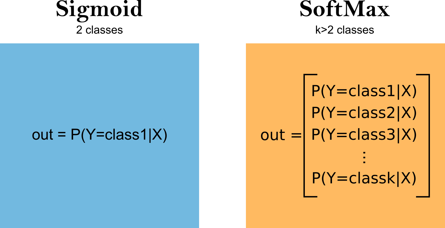
The Difference:

Linear: Output is to −∞ to +∞.
Logistic: Output is Probability ( 0 to 1).

The 2 Changes:

Component	Linear Regression	Logistic Regression
1. The Math	$y= wx + b$	$y = \sigma(wx + b)$
2. The Loss	`MSELoss` (Mean Squared Error)	`BCELoss` (Binary Cross Entropy)

# Example binary classification data
X = torch.tensor([[0.0], [1.0], [2.0], [3.0]], dtype=torch.float32)
y = torch.tensor([[0.0], [0.0], [1.0], [1.0]], dtype=torch.float32)  # Labels: 0 or 1

class LogisticRegression(nn.Module):
    def __init__(self):
        super().__init__()
        self.linear = nn.Linear(1, 1)
    def forward(self, x):
        return self.linear(x)

# The loss function handles the sigmoid internally
criterion = nn.BCEWithLogitsLoss()

# Initialize model
model = LogisticRegression()

# Optimizer remains exactly the same
optimizer = torch.optim.SGD(model.parameters(), lr=0.01)

for epoch in range(200):
    logits = model(X)
    loss = criterion(logits, y)
    loss.backward()
    optimizer.step()
    optimizer.zero_grad()
    if epoch % 20 == 0:
        print(f"Epoch {epoch}: loss={loss.item():.4f}")

Epoch 0: loss=0.9765
Epoch 20: loss=0.8328
Epoch 40: loss=0.7302
Epoch 60: loss=0.6593
Epoch 80: loss=0.6104
Epoch 100: loss=0.5759
Epoch 120: loss=0.5508
Epoch 140: loss=0.5317
Epoch 160: loss=0.5167
Epoch 180: loss=0.5043

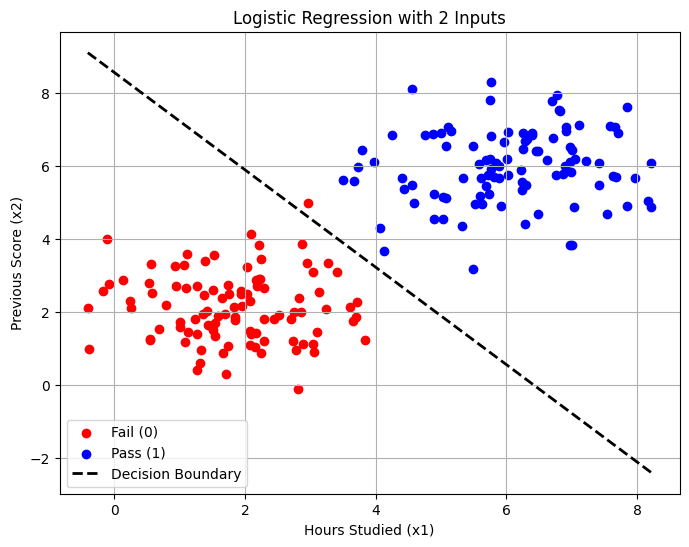
Logistic Regression with Two Inputs¶

In this scenario, we will predict if a student Passes (1) or Fails (0) based on two input features:

: $x_{1}$ Hours Studied
: $x_{2}$ Previous Test Score

1. The Math¶

Since we have two inputs ( $x_{1}, x_{2}$ ), our model learns a weighted sum plus a bias. The equation for the “logit” (before the sigmoid squashing) is:

y = w_{1}*x_{1} + w_{2}*x_{2}

(1)

2. The PyTorch Implementation¶

import torch
import torch.nn as nn
import torch.optim as optim
import matplotlib.pyplot as plt
import numpy as np

# --- 1. GENERATE SYNTHETIC DATA ---
# We create two clusters of data:
# Class 0 (Fail): Centered at (2, 2)
# Class 1 (Pass): Centered at (6, 6)
n_samples = 100
class_0 = torch.randn(n_samples, 2) + 2  
class_1 = torch.randn(n_samples, 2) + 6 

# Combine them
X = torch.cat([class_0, class_1], dim=0) # Shape: [200, 2] -> 2 Inputs!
y = torch.cat([torch.zeros(n_samples, 1), torch.ones(n_samples, 1)], dim=0)

print(X)
print(y)

tensor([[ 2.7807,  0.9569],
        [ 1.2654,  1.3800],
        [ 1.3522,  1.9388],
        [ 1.4730,  1.5970],
        [ 0.2404,  2.2981],
        [ 2.1749,  2.8792],
        [ 2.7312,  1.1890],
        [ 2.8652,  3.8674],
        [ 1.9424,  2.4870],
        [ 2.0797,  1.4841],
        [ 3.2401,  2.0771],
        [ 1.6590,  0.8739],
        [-0.1771,  2.5757],
        [-0.0757,  2.7612],
        [ 1.8462,  1.7691],
        [ 0.5278,  2.7960],
        [ 0.9302,  3.2490],
        [ 0.6902,  1.5390],
        [ 2.2501,  3.4632],
        [ 1.7121,  0.2944],
        [ 3.2751,  3.3384],
        [ 0.2618,  2.0997],
        [ 2.8561,  1.9894],
        [ 0.7829,  2.1906],
        [ 1.4282,  1.6493],
        [ 1.8273,  2.1232],
        [ 2.1886,  2.7055],
        [ 1.2406,  1.7956],
        [ 2.0708,  1.0981],
        [ 2.0299,  2.4871],
        [ 1.1111,  3.5885],
        [ 1.3778,  2.4542],
        [ 2.0849,  1.3890],
        [ 0.9474,  2.6981],
        [ 1.5268,  3.5509],
        [ 1.3290,  0.9418],
        [ 2.9593,  4.9950],
        [ 1.7448,  2.7436],
        [ 2.2115,  2.8997],
        [ 3.1048,  1.4557],
        [ 0.5412,  1.2467],
        [ 2.5263,  1.9146],
        [ 2.2269,  2.9000],
        [ 2.8869,  1.1191],
        [ 1.1338,  1.4415],
        [ 3.0588,  0.9105],
        [ 2.4402,  1.8090],
        [ 0.5625,  3.3157],
        [ 3.7005,  1.8681],
        [ 1.8397,  1.8455],
        [ 3.8375,  1.2173],
        [ 1.3067,  0.5920],
        [ 2.1565,  1.0480],
        [ 2.0862,  4.1322],
        [ 2.2921,  1.7973],
        [ 1.3861,  3.3978],
        [ 1.9496,  2.1574],
        [-0.1087,  4.0118],
        [ 1.4148,  2.0137],
        [ 3.7180,  2.2580],
        [ 1.5145,  1.4898],
        [ 2.0288,  3.2336],
        [ 1.5906,  1.8727],
        [ 1.0952,  2.6581],
        [ 1.0041,  1.5747],
        [ 2.0799,  2.3023],
        [ 3.1318,  2.5393],
        [ 2.6958,  1.8130],
        [-0.3868,  0.9692],
        [-0.4057,  2.1033],
        [ 1.5437,  1.3454],
        [ 1.7498,  2.4864],
        [ 1.2611,  2.6964],
        [ 1.5437,  1.6827],
        [ 1.0679,  3.2967],
        [ 1.0842,  1.1706],
        [ 0.1286,  2.8742],
        [ 0.5771,  2.5055],
        [ 2.2126,  3.8337],
        [ 0.5456,  1.2154],
        [ 1.6878,  1.9532],
        [ 2.2457,  0.8747],
        [ 2.2828,  1.2071],
        [ 3.4145,  3.0984],
        [ 2.8099, -0.1245],
        [ 1.7451,  1.0522],
        [ 1.0003,  1.7144],
        [ 3.6443,  1.7499],
        [ 2.1646,  1.4160],
        [ 1.9333,  2.5643],
        [ 3.0441,  1.1266],
        [ 2.2872,  2.6436],
        [ 1.6495,  2.3840],
        [ 2.8203,  2.3818],
        [ 3.0333,  3.0972],
        [ 2.7458,  1.9857],
        [ 1.2655,  0.3953],
        [ 3.6094,  2.1249],
        [ 2.9548,  3.3455],
        [ 1.5150,  2.6045],
        [ 3.7857,  6.4392],
        [ 3.6625,  5.5940],
        [ 5.7521,  6.1945],
        [ 4.4293,  5.3580],
        [ 5.8074,  5.6974],
        [ 5.3315,  5.6726],
        [ 6.8723,  5.7846],
        [ 6.9871,  5.8350],
        [ 6.9957,  3.8220],
        [ 5.6086,  5.6671],
        [ 5.8446,  6.0946],
        [ 4.2474,  6.8557],
        [ 6.0170,  6.9297],
        [ 6.2572,  6.4598],
        [ 6.2842,  6.6972],
        [ 4.7554,  6.8494],
        [ 7.6364,  5.7243],
        [ 5.7109,  5.7686],
        [ 5.4907,  6.5571],
        [ 4.9998,  6.9062],
        [ 4.5856,  4.9981],
        [ 5.1441,  6.9500],
        [ 7.5830,  7.1100],
        [ 7.8474,  7.6331],
        [ 7.2165,  6.1306],
        [ 4.5499,  5.4932],
        [ 5.0792,  5.1294],
        [ 8.2186,  6.0854],
        [ 5.0997,  7.0790],
        [ 5.4948,  3.1738],
        [ 5.3260,  4.3472],
        [ 4.0700,  4.2938],
        [ 6.3956,  6.9145],
        [ 7.0522,  6.2021],
        [ 6.0296,  5.7655],
        [ 4.8838,  5.2234],
        [ 6.2170,  5.9050],
        [ 5.8828,  5.9960],
        [ 6.3064,  5.4687],
        [ 6.7781,  7.9646],
        [ 3.9667,  6.1084],
        [ 5.5123,  4.9621],
        [ 6.3912,  6.8653],
        [ 5.7624,  8.3073],
        [ 7.1066,  7.1177],
        [ 4.8869,  4.5464],
        [ 7.5401,  4.6957],
        [ 6.8988,  6.0049],
        [ 6.4816,  6.4244],
        [ 5.6926,  6.1746],
        [ 6.9662,  6.1220],
        [ 6.2427,  5.3527],
        [ 6.9751,  3.8226],
        [ 6.4883,  4.6863],
        [ 6.8194,  7.4993],
        [ 4.4013,  5.6609],
        [ 7.0350,  4.8754],
        [ 6.2597,  6.9106],
        [ 7.4232,  6.0786],
        [ 6.2419,  5.5541],
        [ 6.7161,  6.7732],
        [ 8.2127,  4.8734],
        [ 6.9063,  6.9537],
        [ 5.5941,  5.1871],
        [ 7.8512,  4.9156],
        [ 6.3103,  6.7501],
        [ 5.7707,  6.8350],
        [ 5.7284,  5.2368],
        [ 6.9160,  7.0620],
        [ 5.9663,  6.6604],
        [ 7.7031,  6.9172],
        [ 5.9187,  4.8951],
        [ 4.8831,  6.8785],
        [ 6.6983,  7.7729],
        [ 6.7587,  5.7501],
        [ 8.1726,  5.0348],
        [ 5.6301,  4.9507],
        [ 6.8040,  7.5296],
        [ 6.4454,  6.4056],
        [ 7.6730,  5.6997],
        [ 6.0009,  6.1950],
        [ 5.7656,  5.9248],
        [ 5.6843,  5.4466],
        [ 5.0301,  5.1399],
        [ 7.9705,  5.6639],
        [ 4.5494,  8.1087],
        [ 6.6171,  6.1550],
        [ 7.6608,  7.0626],
        [ 5.0680,  6.5455],
        [ 7.0102,  6.4279],
        [ 5.7452,  7.8249],
        [ 3.4912,  5.6253],
        [ 5.0268,  4.5366],
        [ 7.4137,  5.4679],
        [ 5.8802,  5.6713],
        [ 6.9772,  6.5330],
        [ 5.5748,  6.0651],
        [ 6.2872,  4.3989],
        [ 3.7209,  5.9790],
        [ 4.1251,  3.6739]])
tensor([[0.],
        [0.],
        [0.],
        [0.],
        [0.],
        [0.],
        [0.],
        [0.],
        [0.],
        [0.],
        [0.],
        [0.],
        [0.],
        [0.],
        [0.],
        [0.],
        [0.],
        [0.],
        [0.],
        [0.],
        [0.],
        [0.],
        [0.],
        [0.],
        [0.],
        [0.],
        [0.],
        [0.],
        [0.],
        [0.],
        [0.],
        [0.],
        [0.],
        [0.],
        [0.],
        [0.],
        [0.],
        [0.],
        [0.],
        [0.],
        [0.],
        [0.],
        [0.],
        [0.],
        [0.],
        [0.],
        [0.],
        [0.],
        [0.],
        [0.],
        [0.],
        [0.],
        [0.],
        [0.],
        [0.],
        [0.],
        [0.],
        [0.],
        [0.],
        [0.],
        [0.],
        [0.],
        [0.],
        [0.],
        [0.],
        [0.],
        [0.],
        [0.],
        [0.],
        [0.],
        [0.],
        [0.],
        [0.],
        [0.],
        [0.],
        [0.],
        [0.],
        [0.],
        [0.],
        [0.],
        [0.],
        [0.],
        [0.],
        [0.],
        [0.],
        [0.],
        [0.],
        [0.],
        [0.],
        [0.],
        [0.],
        [0.],
        [0.],
        [0.],
        [0.],
        [0.],
        [0.],
        [0.],
        [0.],
        [0.],
        [1.],
        [1.],
        [1.],
        [1.],
        [1.],
        [1.],
        [1.],
        [1.],
        [1.],
        [1.],
        [1.],
        [1.],
        [1.],
        [1.],
        [1.],
        [1.],
        [1.],
        [1.],
        [1.],
        [1.],
        [1.],
        [1.],
        [1.],
        [1.],
        [1.],
        [1.],
        [1.],
        [1.],
        [1.],
        [1.],
        [1.],
        [1.],
        [1.],
        [1.],
        [1.],
        [1.],
        [1.],
        [1.],
        [1.],
        [1.],
        [1.],
        [1.],
        [1.],
        [1.],
        [1.],
        [1.],
        [1.],
        [1.],
        [1.],
        [1.],
        [1.],
        [1.],
        [1.],
        [1.],
        [1.],
        [1.],
        [1.],
        [1.],
        [1.],
        [1.],
        [1.],
        [1.],
        [1.],
        [1.],
        [1.],
        [1.],
        [1.],
        [1.],
        [1.],
        [1.],
        [1.],
        [1.],
        [1.],
        [1.],
        [1.],
        [1.],
        [1.],
        [1.],
        [1.],
        [1.],
        [1.],
        [1.],
        [1.],
        [1.],
        [1.],
        [1.],
        [1.],
        [1.],
        [1.],
        [1.],
        [1.],
        [1.],
        [1.],
        [1.],
        [1.],
        [1.],
        [1.],
        [1.],
        [1.],
        [1.]])


# --- 2. DEFINE THE MODEL ---
class LogisticRegression2D(nn.Module):
    def __init__(self):
        super().__init__()
        # Two Inputs (Hours, Score) -> One Output (Logit)
        self.linear = nn.Linear(in_features=2, out_features=1)

    def forward(self, x):
        # We return logits (raw values) for stability
        return self.linear(x)


# Initialize
model = LogisticRegression2D()
criterion = nn.BCEWithLogitsLoss() # Handles the Sigmoid internally
optimizer = optim.SGD(model.parameters(), lr=0.1)


# --- 3. TRAIN ---
epochs = 1000
for epoch in range(epochs):
    # Forward
    logits = model(X)
    loss = criterion(logits, y)
    
    # Backward
    loss.backward()
    optimizer.step()
    optimizer.zero_grad()
    
    if (epoch+1) % 200 == 0:
        print(f"Epoch {epoch+1}, Loss: {loss.item():.4f}")

Epoch 200, Loss: 0.2375
Epoch 400, Loss: 0.1504
Epoch 600, Loss: 0.1134
Epoch 800, Loss: 0.0929
Epoch 1000, Loss: 0.0798


# --- 4. VISUALIZE THE RESULTS ---
# Extract learned weights (w1, w2) and bias (b)
w1, w2 = model.linear.weight.detach().numpy()[0]
b = model.linear.bias.detach().item()

# Plot Data Points
plt.figure(figsize=(8, 6))
plt.scatter(X[:n_samples, 0], X[:n_samples, 1], c='red', label='Fail (0)')
plt.scatter(X[n_samples:, 0], X[n_samples:, 1], c='blue', label='Pass (1)')

# Calculate Decision Boundary Line
# The line is defined by: w1*x1 + w2*x2 + b = 0
# Solve for x2: x2 = -(w1*x1 + b) / w2
x1_plot = np.array([X[:, 0].min(), X[:, 0].max()])
x2_plot = -(w1 * x1_plot + b) / w2

plt.plot(x1_plot, x2_plot, 'k--', linewidth=2, label='Decision Boundary')
plt.xlabel('Hours Studied (x1)')
plt.ylabel('Previous Score (x2)')
plt.legend()
plt.title('Logistic Regression with 2 Inputs')
plt.grid(True)
plt.show()

3. Key Takeaways¶

The Input Shape: Notice nn.Linear(2, 1). The 2 corresponds directly to our two columns of data ( $x_{1}$ and $x_{2}$ ).
The Weights: The model learns two weights:

$w_{1}$ : How much “Hours Studied” matters.
$w_{2}$ : How much “Previous Score” matters.

The Line: Even though we use a curve (Sigmoid) to predict probability, the boundary that splits the two classes is a Straight Line. This is why it is still a “Linear” Classifier.

Part 6: MNIST (Handwritten Digits)¶

MNIST is the standard “Hello World” for Deep Learning.

However, there is a major twist: MNIST has 10 classes (digits 0–9), not just 2.

This means we are upgrading from Binary Logistic Regression (Pass/Fail) to Multinomial Logistic Regression (often called Softmax Regression).

1. The Conceptual Shift¶

Input: An image is a grid. To put it into nn.Linear, we must flatten it into a single long vector of 784 numbers ().
Output: We don’t output 1 number; we output 10 numbers (scores for each digit).
Activation: We replace Sigmoid (Yes/No) with Softmax (Probability distribution across 10 options).

2. The PyTorch Implementation¶

This script downloads the data, trains the model, and visualizes predictions.

Let’s load the data

import torch
import torch.nn as nn
import torch.optim as optim
import torchvision
import torchvision.transforms as transforms
import matplotlib.pyplot as plt

# --- 1. PREPARE DATA ---

# Download MNIST Dataset
train_dataset = torchvision.datasets.MNIST(root='./data', train=True, download=True, transform=transforms.ToTensor())
test_dataset = torchvision.datasets.MNIST(root='./data', train=False, download=True, transform=transforms.ToTensor())

torchvision.datasets.MNIST loads the MNIST handwritten digits dataset.
root='./data' tells PyTorch where to store (or find) the data.
train=True loads the training set (60,000 images); train=False loads the test set (10,000 images).
download=True will download the data if it’s not already present.
transform=transforms.ToTensor() converts each image from a PIL image (or numpy array) to a PyTorch tensor, which is required for model training.

train_dataset

Dataset MNIST
    Number of datapoints: 60000
    Root location: ./data
    Split: Train
    StandardTransform
Transform: ToTensor()

Let’s print out some images

import matplotlib.pyplot as plt

fig, axes = plt.subplots(1, 10, figsize=(15, 2))
for i in range(10):
    image, label = train_dataset[i]
    axes[i].imshow(image.squeeze(), cmap='gray')
    axes[i].set_title(label)
    axes[i].axis('off')
plt.show()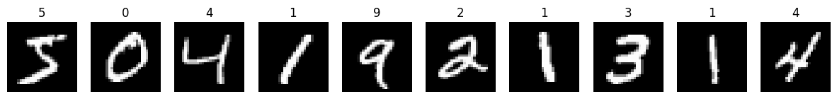

# Data Loaders (Batches of 64 images)
train_loader = torch.utils.data.DataLoader(train_dataset, batch_size=64, shuffle=True)
test_loader = torch.utils.data.DataLoader(test_dataset, batch_size=64, shuffle=False)

torch.utils.data.DataLoader creates an iterator that loads data in batches.
batch_size=64 means each batch contains 64 images and labels.
shuffle=True (for training) randomly shuffles the data at each epoch, which helps the model generalize better.
shuffle=False (for testing) keeps the data in order for consistent evaluation.

Batch Size¶

Imagine you have to eat a giant bowl of 10,000 grains of rice (your data). You have a few options for how to eat it:

Batch Size = 1 (Stochastic Gradient Descent): You eat one single grain of rice, swallow, and decide if you are full.
- Pros: You get feedback instantly.
- Cons: It takes forever. The feedback is noisy (one bad grain ruins the vibe).
Batch Size = 10,000 (Full Batch Learning): You try to shove the entire bowl into your mouth at once.
- Pros: The feedback is perfectly accurate (average of everything).
- Cons: You will choke (Run out of RAM/Memory). It’s very slow to calculate.
Batch Size = 32 or 64 (Mini-Batch Gradient Descent): You use a spoon. You scoop up 32 grains, eat them, digest, and repeat.
- The Sweet Spot: This is what we actually use. It offers a balance of speed and accuracy.

In Technical Terms:

Batch Size is the number of training examples utilized in one iteration.
The model looks at these 32 examples, calculates the average loss, and updates the weights once.

Epoch vs. Iteration¶

This is where people often get confused:

Dataset: 1,000 images.
Batch Size: 100.

The Math:

1 Iteration: The model sees 100 images and updates weights once.
1 Epoch: The model has seen all 1,000 images.
Calculations:
It takes 10 Iterations (1,000 / 100) to complete 1 Epoch.

If you train for 5 Epochs, the model updates its weights 50 times (5 epochs 10 batches).

In Scikit-Learn, model.fit(X, y) does all this automatically (usually as a Full Batch). In PyTorch, if you don’t use a DataLoader, you are likely doing Full Batch training, which works for tiny datasets (like 100 samples) but will crash your computer with real data (like 100,000 samples). The DataLoader is the bridge to “Real AI.”

Flatten images¶

Think of nn.Linear (the Fully Connected Layer) as a very strict accountant. It refuses to look at spreadsheets (2D Grids); it only looks at long lists of numbers (1D Vectors).

Flattening is simply the process of taking our 2D image and unrolling it into that long list so the layer can process it.

1. The Visual Concept¶

Imagine you have a tiny image that is only pixels (9 pixels total). It looks like a tic-tac-toe board.


A	D	G
B	E	H
C	F	I

The neural network cannot ingest this square. It needs a single line. So, we take the first row, then glue the second row to the end of it, and then the third row.

[A,B,C,D,E,F,G,H,I]

Now, applying this to MNIST:

Original Image: 28 pixels tall, 28 pixels wide.
Flattened Vector: 28 x 28 = 784 numbers in a straight line.

2. Why do we do this?¶

The math inside the layer is the Dot Product: . This formula pairs one weight () with one input pixel (). It doesn’t care if pixel was originally “above” pixel . It just treats them all as separate features in a bucket.

The reason we flatten a 2D image into 1D is a mismatch between the data format (a grid) and the math tool (Linear Regression/nn.Linear).

Here is the breakdown of why this happens and what we lose in the process.

1. The Compatibility Problem¶

The nn.Linear layer is designed to process Flat Lists (Vectors), not Grids (Matrices).

The Tool (nn.Linear): Think of a Linear Layer as a standard Excel spreadsheet equation. It expects a single row of input features: [Age, Height, Weight, Income].
The Data (Image): An image is a 2D grid: 28 rows x 28 columns.

To feed the image into the equation, we must “unroll” the rows and glue them together into one long single row. We treat every pixel not as a point in a picture, but as a separate, independent statistic.

2. The Mathematical Reason (Dot Product)¶

The math inside a Linear Layer is a weighted sum:

y = w_1 x_1 + w_2 x_2 + w_3 x_3 + \cdots + b

(2)

This formula doesn’t have a concept of “up,” “down,” “left,” or “right.” It only understands “Item 1,” “Item 2,” “Item 3.”

Pixel (0,1) becomes $x_{1}$
Pixel (0,1) becomes $x_{2}$
Pixel (10,10) becomes $x_{290}$

The layer learns a unique weight ( $w$ ) for every single pixel position, but it treats them all as independent variables, just like “Age” and “Income” are independent variables.

3. The Code (`.view`)¶

In PyTorch, we use .view() (or .reshape()) to do this.

# Take one image from the training set
image, label = train_dataset[0]

print("Original shape:", image.shape)  # Should be [1, 28, 28]

# Flatten the image to a 1D vector of length 784
flattened = image.view(-1)
print("Flattened shape:", flattened.shape)  # Should be [784]

# Optionally, show the first 20 values
print("First 20 pixel values:", flattened[:20])

Original shape: torch.Size([1, 28, 28])
Flattened shape: torch.Size([784])
First 20 pixel values: tensor([0., 0., 0., 0., 0., 0., 0., 0., 0., 0., 0., 0., 0., 0., 0., 0., 0., 0., 0., 0.])

import matplotlib.pyplot as plt

# Display the original image
plt.figure(figsize=(8, 2))

plt.subplot(1, 2, 1)
plt.imshow(image.squeeze(), cmap='gray')
plt.title(f"Label: {label}")
plt.axis('off')

# Display the flattened image as a row vector
plt.subplot(1, 2, 2)
plt.imshow(flattened.unsqueeze(0), cmap='gray', aspect='auto')
plt.title("Flattened (1x784)")
plt.xlabel("Pixel Index")
plt.yticks([])
plt.tight_layout()
plt.show()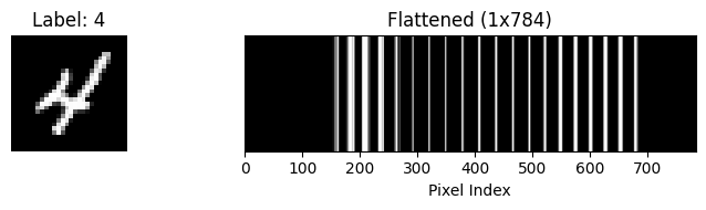

What do the numbers mean?

784: This is the new size we want for the columns ().
-1: This is a special instruction to PyTorch that means “You figure this number out.”
Since we have a total of numbers, and we just told PyTorch to put 784 in each row, PyTorch calculates: .
So, -1 automatically preserves your Batch Size (64).

Result: The shape transforms from [64, 1, 28, 28] [64, 784].

The Consequence¶

Flattening destroys spatial information. Once you flatten the image, the model no longer knows that the top-left pixel is near the pixel below it. It treats them as completely unrelated inputs.

This is why we eventually switch to Convolutional Neural Networks (CNNs) later in the course—CNNs can read the 2D grid directly without flattening it first.


# --- 2. DEFINE THE MODEL (Multinomial Logistic Regression) ---
class MNISTLogisticModel(nn.Module):
    def __init__(self):
        super().__init__()
        # Input: 28x28 = 784 pixels
        # Output: 10 Classes (Digits 0-9)
        self.linear = nn.Linear(in_features=784, out_features=10)

    def forward(self, x):
        # FLATTEN: Reshape image [Batch, 1, 28, 28] -> [Batch, 784]
        x = x.view(-1, 784) 
        
        # We return Raw Logits (CrossEntropyLoss handles the Softmax)
        return self.linear(x)


model = MNISTLogisticModel()

# --- 3. LOSS & OPTIMIZER ---
# CrossEntropyLoss = LogSoftmax + Negative Log Likelihood
# It is the standard loss for Multi-Class problems
criterion = nn.CrossEntropyLoss()
optimizer = optim.SGD(model.parameters(), lr=0.01)


# --- 4. TRAINING LOOP ---
print("Training Started...")
for epoch in range(5):  # 5 Epochs is enough for a simple linear model
    running_loss = 0.0
    for images, labels in train_loader:
        # 1. Forward
        outputs = model(images)
        
        # 2. Loss
        loss = criterion(outputs, labels)
        
        # 3. Backward
        loss.backward()
        
        # 4. Update
        optimizer.step()
        optimizer.zero_grad()
        
        running_loss += loss.item()
    
    print(f"Epoch {epoch+1}, Loss: {running_loss/len(train_loader):.4f}")

print("Training Finished.")

Training Started...
Epoch 1, Loss: 0.9786
Epoch 2, Loss: 0.5515
Epoch 3, Loss: 0.4721
Epoch 4, Loss: 0.4335
Epoch 5, Loss: 0.4093
Training Finished.


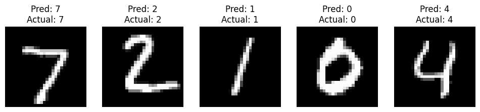
# --- 5. TEST & VISUALIZE ---
# Get a batch of test images
dataiter = iter(test_loader)
images, labels = next(dataiter)

# Make predictions
outputs = model(images)
_, predicted = torch.max(outputs, 1) # Get the index of the highest score

# Plot the first 5 images and their predictions
fig, axes = plt.subplots(1, 5, figsize=(12, 3))
for i in range(5):
    image = images[i].squeeze().numpy()
    axes[i].imshow(image, cmap='gray')
    axes[i].set_title(f"Pred: {predicted[i].item()}\nActual: {labels[i].item()}")
    axes[i].axis('off')
plt.show()

Part 6: Lab Activities¶

“Break the Loop”: Comment out optimizer.zero_grad() and watch the loss explode.
“Shape Detective”: Calculate the in_features for an image classifier (e.g., 28x28 pixels = 784 inputs).
“Refactoring Challenge”: Given the manual w and b code from Part 4, rewrite it using nn.Linear.

Part 1: The “Black Box” vs. The “Glass Box”¶

The scikit-learn way¶

The PyTorch way¶

Part 2: The Prerequisite – OOP for Deep Learning¶

The Concept¶

The Analogy: The Robot Factory¶

Inheritance: BattleBot is a Robot, but with extra features¶

Part 3: Implementation – The PyTorch OOP Way¶

1. The Layer: nn.Linear¶

2. The Model Class¶

3. The Training Loop¶

Part 4: Comparison with the non-OOP way from the last class¶

Part 5: Extension – Logistic Regression¶

Logistic Regression with Two Inputs¶

1. The Math¶

2. The PyTorch Implementation¶

3. Key Takeaways¶

Part 6: MNIST (Handwritten Digits)¶

1. The Conceptual Shift¶

2. The PyTorch Implementation¶

Batch Size¶

Epoch vs. Iteration¶

Flatten images¶

1. The Visual Concept¶

2. Why do we do this?¶

1. The Compatibility Problem¶

2. The Mathematical Reason (Dot Product)¶

3. The Code (.view)¶

The Consequence¶

Part 6: Lab Activities¶

1. The Layer: `nn.Linear`¶

3. The Code (`.view`)¶