Before we dive in: You’ve already taught a CNN to recognise images by learning spatial patterns. Now we’ll teach a network to read — to understand sequences by learning temporal patterns. We work data-first: start with real text, define what we want to predict, then build the machinery step by step.
Learning Objectives
By the end of this tutorial you will be able to:
Explain why MLPs fail on sequential data and what problem RNNs solve.
Describe the main text prediction tasks: next character, next word, and sentiment classification.
Convert raw text to numbers: tokenisation, vocabulary, and
nn.Embedding.Build input/target pairs for sequence prediction using a sliding window.
Implement an RNN cell from scratch and explain the role of the hidden state.
Train a character-level language model and generate text.
Prerequisites (Tutorial 7 Recap)
In Tutorial 7 you:
Loaded pre-trained CNNs (AlexNet, ResNet18) from
torchvision.models.Froze backbone weights and fine-tuned only the classifier head.
Today we shift from images to text sequences — data where order matters.
# ── Setup ──────────────────────────────────────────────────────────────
import random
from collections import Counter

import torch
import torch.nn as nn
import torch.nn.functional as F
import torch.optim as optim
from torch.utils.data import DataLoader, TensorDataset, Dataset

import numpy as np
import matplotlib.pyplot as plt

import plotly.graph_objects as go
from plotly.subplots import make_subplots

torch.manual_seed(42)
np.random.seed(42)
random.seed(42)

if torch.backends.mps.is_available():
    device = torch.device('mps')
elif torch.cuda.is_available():
    device = torch.device('cuda')
else:
    device = torch.device('cpu')

print(f'Using device: {device}')
Using device: mps
Part 1 — Why Do We Need RNNs? 🧠
The Problem with MLPs on Text
In Tutorial 3 and 4 you learned that an MLP takes a fixed-size input vector and maps it to an output. Every input position is treated independently — there’s no built-in concept of before or after.
This is a serious problem for language. Consider:
“I grew up in France. I went to school there. I learned the culture. I speak fluent ___.”
The answer is French — but to know that, you need to remember a word from much earlier in the sequence. A traditional MLP can only look at the tokens you explicitly place in its input window. If the useful clue sits outside that window, the model never sees it.
How the Supervised Data Looks
For next-token prediction, a fixed-window MLP and an RNN are trained on different input structures:
MLP:
last k tokens -> next tokenRNN:
token 1, then token 2, then token 3, ... -> updated hidden state -> next token
That difference is the whole point: the MLP has a short, hard cutoff on memory, while the RNN carries a running summary forward through time.
# ── Part 1: How MLP and RNN training examples are structured ─────────────
tokens = ['I', 'grew', 'up', 'in', 'France', '.', 'I', 'speak', 'fluent', '___']
MLP_WINDOW = 3

print('Fixed-window MLP training pairs (window = 3 tokens):')
print()
for i in range(MLP_WINDOW, len(tokens)):
    context = tokens[i - MLP_WINDOW:i]
    target = tokens[i]
    print(f'  input={context!r:<30} -> target={target!r}')

print()
print("Prediction for the blank:")
print(f"  MLP sees only: {tokens[-1-MLP_WINDOW:-1]}")
print(f"  Key clue 'France' is {len(tokens) - 1 - tokens.index('France')} positions back — outside the window.")
print()
print('RNN view of the same prediction:')
for step, token in enumerate(tokens[:-1], start=1):
    prefix = tokens[:step]
    print(f'  step {step:>2}: prefix={prefix!r}')
print()
print("The RNN receives the whole prefix one token at a time, so 'France' can influence the prediction.")
Fixed-window MLP training pairs (window = 3 tokens):
input=['I', 'grew', 'up'] -> target='in'
input=['grew', 'up', 'in'] -> target='France'
input=['up', 'in', 'France'] -> target='.'
input=['in', 'France', '.'] -> target='I'
input=['France', '.', 'I'] -> target='speak'
input=['.', 'I', 'speak'] -> target='fluent'
input=['I', 'speak', 'fluent'] -> target='___'
Prediction for the blank:
MLP sees only: ['I', 'speak', 'fluent']
Key clue 'France' is 5 positions back — outside the window.
RNN view of the same prediction:
step 1: prefix=['I']
step 2: prefix=['I', 'grew']
step 3: prefix=['I', 'grew', 'up']
step 4: prefix=['I', 'grew', 'up', 'in']
step 5: prefix=['I', 'grew', 'up', 'in', 'France']
step 6: prefix=['I', 'grew', 'up', 'in', 'France', '.']
step 7: prefix=['I', 'grew', 'up', 'in', 'France', '.', 'I']
step 8: prefix=['I', 'grew', 'up', 'in', 'France', '.', 'I', 'speak']
step 9: prefix=['I', 'grew', 'up', 'in', 'France', '.', 'I', 'speak', 'fluent']
The RNN receives the whole prefix one token at a time, so 'France' can influence the prediction.
# ── Part 1: Context Window Visualisation ───────────────────────────────
sentence = ['I', 'grew', 'up', 'in', 'France', '.', 'I', 'speak', 'fluent', '___']
mlp_weights = np.array([0.02, 0.02, 0.03, 0.05, 0.01, 0.02, 0.15, 0.25, 0.40, 0.0])
rnn_weights = np.array([0.05, 0.08, 0.07, 0.10, 0.30, 0.05, 0.10, 0.10, 0.10, 0.0])

colors_mlp = ['#e74c3c' if w > 0.1 else '#fadbd8' for w in mlp_weights]
colors_rnn = ['#27ae60' if w > 0.1 else '#d5f5e3' for w in rnn_weights]

fig = make_subplots(
    rows=1, cols=2,
    subplot_titles=('MLP: only nearby words matter', 'RNN: long-range context remembered')
)
fig.add_trace(
    go.Bar(x=sentence, y=mlp_weights, marker_color=colors_mlp, name='MLP',
           hovertemplate='Word: %{x}<br>Influence: %{y:.2f}<extra></extra>'),
    row=1, col=1)
fig.add_trace(
    go.Bar(x=sentence, y=rnn_weights, marker_color=colors_rnn, name='RNN',
           hovertemplate='Word: %{x}<br>Influence: %{y:.2f}<extra></extra>'),
    row=1, col=2)
fig.update_layout(
    title_text='How Much Each Word Influences the Prediction of "___"',
    height=380, showlegend=False, template='plotly_white')
fig.update_yaxes(title_text='Influence Weight', range=[0, 0.55])
fig.show()
print("The RNN gives high weight to 'France' (the key context word), which the MLP misses.")The RNN gives high weight to 'France' (the key context word), which the MLP misses.
Checkpoint
MCQ 1: Why do MLPs struggle with sequential text data?
A. They use too many parameters and overfit quickly.
B. Inputs are treated independently, so there is no memory of previous tokens.
C. They cannot handle integer inputs; text must first be converted to floats.
D. They require sequences to be sorted alphabetically before training.
Answer: B — A fixed-window MLP only uses the tokens explicitly placed in the input vector, so sequence memory is limited by that window size.
Part 2 — The Data: What Are We Working With? 📄
Before writing any model code, let’s look at the actual data and the tasks we want to solve.
Our Training Corpus
We’ll use a nursery rhyme as our text corpus — small enough to read in full, which makes it easy to inspect what the model is learning.
Three Prediction Tasks
| # | Task | Input | Output | Model |
|---|---|---|---|---|
| 1 | Next-character prediction | 'mary had a litt' | 'l' | CharRNN / CharLSTM |
| 2 | Next-word prediction | ['mary', 'had', 'a'] | 'little' | (illustrated) |
| 3 | Sentiment classification | 'this film was fantastic' | positive | SentimentLSTM |
All three share one challenge: order matters — you can’t shuffle the words and still answer correctly. The rest of this tutorial builds the tools to solve each task.
# ── Part 2: The Text Corpus and Three Prediction Tasks ────────────────
# Dataset 1: Nursery rhyme — our training corpus
TEXT = (
    'mary had a little lamb little lamb little lamb '
    'mary had a little lamb its fleece was white as snow '
    'and everywhere that mary went mary went mary went '
    'and everywhere that mary went the lamb was sure to go '
    'it followed her to school one day school one day school one day '
    'it followed her to school one day which was against the rules'
)

print('=== CORPUS ===')
print(TEXT)
print(f'\nLength: {len(TEXT)} characters,  unique: {len(set(TEXT))}')

print('\n=== TASK 1: Next-Character Prediction ===')
print('Given a sequence of characters, predict the next one:')
for start in [0, 15, 30]:
    prefix = TEXT[start:start + 15]
    target = TEXT[start + 15]
    print(f'  {repr(prefix)}  →  {repr(target)}')

print('\n=== TASK 2: Next-Word Prediction ===')
words = TEXT.split()
print('Given a sequence of words, predict the next one:')
for i in [0, 4, 8]:
    print(f'  {words[i:i+3]}  →  {repr(words[i+3])}')

print('\n=== TASK 3: Sentiment Classification ===')
print('Given a whole review, predict its sentiment:')
for text, label in [('this film was absolutely wonderful', 'POSITIVE'),
                    ('this film was painfully boring',     'NEGATIVE')]:
    print(f'  {repr(text)}  →  {label}')
=== CORPUS ===
mary had a little lamb little lamb little lamb mary had a little lamb its fleece was white as snow and everywhere that mary went mary went mary went and everywhere that mary went the lamb was sure to go it followed her to school one day school one day school one day it followed her to school one day which was against the rules
Length: 328 characters, unique: 21
=== TASK 1: Next-Character Prediction ===
Given a sequence of characters, predict the next one:
'mary had a litt' → 'l'
'le lamb little ' → 'l'
'lamb little lam' → 'b'
=== TASK 2: Next-Word Prediction ===
Given a sequence of words, predict the next one:
['mary', 'had', 'a'] → 'little'
['lamb', 'little', 'lamb'] → 'little'
['lamb', 'mary', 'had'] → 'a'
=== TASK 3: Sentiment Classification ===
Given a whole review, predict its sentiment:
'this film was absolutely wonderful' → POSITIVE
'this film was painfully boring' → NEGATIVE
# ── Part 2: Visualise the Three Tasks ─────────────────────────────────
fig, axes = plt.subplots(1, 3, figsize=(16, 3.5))
plt.subplots_adjust(wspace=0.35)

# Task 1: next-character
chars1  = list('mary had ') + ['?']
colors1 = ['#AED6F1'] * 9 + ['#F9E79F']
axes[0].bar(range(len(chars1)), [1]*len(chars1), color=colors1, edgecolor='grey', width=0.9)
for i, c in enumerate(chars1):
    axes[0].text(i, 0.5, repr(c), ha='center', va='center', fontsize=9, fontweight='bold')
axes[0].text(9, 1.08, '"a"', ha='center', fontsize=13, color='#1A5276', fontweight='bold')
axes[0].set_title('Task 1 — Next Character\n"mary had " → ?', fontsize=10, fontweight='bold')
axes[0].set_yticks([]); axes[0].set_xticks([]); axes[0].set_ylim(0, 1.4)

# Task 2: next-word
words2  = ['mary', 'had', 'a', '?']
colors2 = ['#A9DFBF'] * 3 + ['#F9E79F']
axes[1].bar(range(len(words2)), [1]*len(words2), color=colors2, edgecolor='grey', width=0.9)
for i, w in enumerate(words2):
    axes[1].text(i, 0.5, w, ha='center', va='center', fontsize=11, fontweight='bold')
axes[1].text(3, 1.08, '"little"', ha='center', fontsize=13, color='#1A5276', fontweight='bold')
axes[1].set_title('Task 2 — Next Word\n"mary had a" → ?', fontsize=10, fontweight='bold')
axes[1].set_yticks([]); axes[1].set_xticks([]); axes[1].set_ylim(0, 1.4)

# Task 3: sentiment
words3  = ['this', 'film', 'was', 'wonderful']
colors3 = ['#D7BDE2'] * 4
axes[2].bar(range(len(words3)), [1]*len(words3), color=colors3, edgecolor='grey', width=0.9)
for i, w in enumerate(words3):
    axes[2].text(i, 0.5, w, ha='center', va='center', fontsize=10, fontweight='bold')
axes[2].annotate('→ POSITIVE', xy=(3.5, 0.5), fontsize=12,
                 color='#1E8449', fontweight='bold', va='center')
axes[2].set_xlim(-0.5, 6)
axes[2].set_title('Task 3 — Sentiment\n"this film was wonderful" → ?', fontsize=10, fontweight='bold')
axes[2].set_yticks([]); axes[2].set_xticks([]); axes[2].set_ylim(0, 1.4)

plt.suptitle('Three Sequence Prediction Tasks — Order Matters in All Cases',
             fontsize=12, fontweight='bold', y=1.03)
plt.show()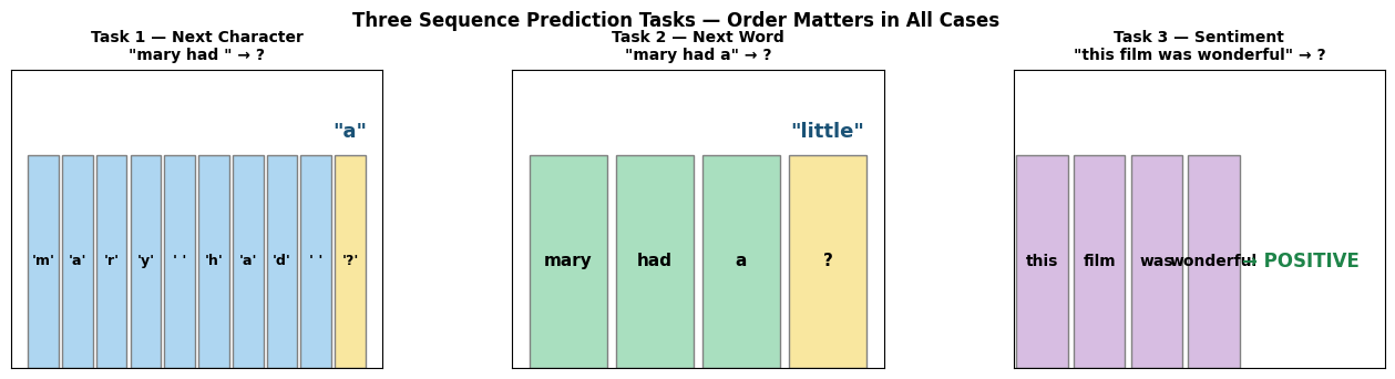
Checkpoint
MCQ 2: Which task requires the model to read the whole sequence before making a single prediction?
A. Task 1 — next-character prediction.
B. Task 2 — next-word prediction.
C. Task 3 — sentiment classification.
D. All three require equal amounts of context.
Answer: C — Sentiment requires one label for the whole review (many-to-one). Tasks 1 and 2 make a prediction at every position (many-to-many). We will build different output heads for these two regimes in Parts 6 and 8.
Part 3 — From Text to Numbers 🔢
Neural networks work with floating-point tensors. To feed them text, we need a pipeline:
raw text → tokenise → build vocabulary → encode as integers → embed as vectorsWe’ll build each step by hand on the nursery rhyme from Part 2.
# ── Part 3: Step 1 — Tokenisation and Vocabulary ──────────────────────
# Split the text into units (tokens). We use characters for our language model.

char_vocab = sorted(set(TEXT))          # all unique characters, sorted
char2idx   = {ch: i for i, ch in enumerate(char_vocab)}
idx2char   = {i: ch for ch, i in char2idx.items()}
VOCAB_SIZE = len(char_vocab)

print(f'Text length      : {len(TEXT)} characters')
print(f'Vocabulary size  : {VOCAB_SIZE} unique characters')
print(f'Vocabulary       : {char_vocab}')
print()

# Word-level for contrast
word_vocab = sorted(set(TEXT.split()))
print(f'Word vocab size  : {len(word_vocab)} unique words')
print(f'Word vocab       : {word_vocab}')
print()
print('We use character-level for the language model.')
print('Real systems use subword tokenisation (BPE/WordPiece) but characters show the ideas cleanly.')
Text length : 328 characters
Vocabulary size : 21 unique characters
Vocabulary : [' ', 'a', 'b', 'c', 'd', 'e', 'f', 'g', 'h', 'i', 'l', 'm', 'n', 'o', 'r', 's', 't', 'u', 'v', 'w', 'y']
Word vocab size : 28 unique words
Word vocab : ['a', 'against', 'and', 'as', 'day', 'everywhere', 'fleece', 'followed', 'go', 'had', 'her', 'it', 'its', 'lamb', 'little', 'mary', 'one', 'rules', 'school', 'snow', 'sure', 'that', 'the', 'to', 'was', 'went', 'which', 'white']
We use character-level for the language model.
Real systems use subword tokenisation (BPE/WordPiece) but characters show the ideas cleanly.
# ── Part 3: Step 2 — Encode Text as Integers ──────────────────────────
sample = 'mary had a'
encoded_sample = [char2idx[c] for c in sample]
decoded_sample = [idx2char[i] for i in encoded_sample]

print(f'Original : {repr(sample)}')
print(f'Encoded  : {encoded_sample}')
print(f'Decoded  : {decoded_sample}')
print()

# Encode the full corpus
encoded_corpus = [char2idx[c] for c in TEXT]
assert ''.join(idx2char[i] for i in encoded_corpus) == TEXT
print(f'Full corpus encoded as {len(encoded_corpus)} integers.')
print(f'First 30 values: {encoded_corpus[:30]}')
Original : 'mary had a'
Encoded : [11, 1, 14, 20, 0, 8, 1, 4, 0, 1]
Decoded : ['m', 'a', 'r', 'y', ' ', 'h', 'a', 'd', ' ', 'a']
Full corpus encoded as 328 integers.
First 30 values: [11, 1, 14, 20, 0, 8, 1, 4, 0, 1, 0, 10, 9, 16, 16, 10, 5, 0, 10, 1, 11, 2, 0, 10, 9, 16, 16, 10, 5, 0]
# ── Part 3: Step 3a — One-Hot Encoding (the naive approach) ────────────
corpus_tensor = torch.tensor(encoded_corpus, dtype=torch.long)
one_hot       = F.one_hot(corpus_tensor, num_classes=VOCAB_SIZE).float()

print(f'One-hot shape: {one_hot.shape}  ({len(encoded_corpus)} chars × {VOCAB_SIZE} vocab)')
print()
print('First 5 characters as one-hot rows:')
for i in range(5):
    ch  = TEXT[i]
    idx = int(corpus_tensor[i])
    print(f'  {repr(ch):4s} (idx={idx:2d})  position {idx} = 1, rest = 0')

print()
bytes_onehot = one_hot.numel() * 4
print(f'Memory for this corpus: {bytes_onehot:,} bytes  ({bytes_onehot/1024:.1f} KB)')
print()
print('Scaling problem:')
print(f'  1M-word corpus × 50k-word vocab → {50_000 * 1_000_000 * 4 / 1e9:.0f} GB just for inputs.')
print('  We need a more compact representation.')
One-hot shape: torch.Size([328, 21]) (328 chars × 21 vocab)
First 5 characters as one-hot rows:
'm' (idx=11) position 11 = 1, rest = 0
'a' (idx= 1) position 1 = 1, rest = 0
'r' (idx=14) position 14 = 1, rest = 0
'y' (idx=20) position 20 = 1, rest = 0
' ' (idx= 0) position 0 = 1, rest = 0
Memory for this corpus: 27,552 bytes (26.9 KB)
Scaling problem:
1M-word corpus × 50k-word vocab → 200 GB just for inputs.
We need a more compact representation.
# ── Part 3: Step 3b — nn.Embedding (dense learned vectors) ────────────
torch.manual_seed(42)
EMBED_DIM = 16
embedding = nn.Embedding(num_embeddings=VOCAB_SIZE, embedding_dim=EMBED_DIM)

embedded = embedding(corpus_tensor)   # (seq_len, EMBED_DIM)
print(f'Embedding table shape  : {embedding.weight.shape}  ({VOCAB_SIZE} tokens × {EMBED_DIM} dims)')
print(f'Embedded corpus shape  : {embedded.shape}')
print(f'Memory: {embedded.numel()*4:,} bytes  (one-hot was {one_hot.numel()*4:,} bytes)')
print(f'Compression: {one_hot.shape[1]/EMBED_DIM:.1f}x fewer numbers per token')
print()

# Plotly heatmap: one-hot vs embedding for first 12 characters
n = 12
oh_np = one_hot[:n].numpy()
em_np = embedded[:n].detach().numpy()
chars = [repr(c) for c in TEXT[:n]]

fig = make_subplots(
    rows=1, cols=2,
    subplot_titles=(f'One-Hot ({VOCAB_SIZE}-dim, sparse)', f'Embedding ({EMBED_DIM}-dim, dense)'))
fig.add_trace(go.Heatmap(
    z=oh_np, x=list(range(VOCAB_SIZE)), y=chars,
    colorscale=[[0, '#f0f4f8'], [1, '#2980b9']], showscale=False,
    hovertemplate='Char %{y}, col %{x}: %{z}<extra></extra>'), row=1, col=1)
fig.add_trace(go.Heatmap(
    z=em_np, x=[f'd{i}' for i in range(EMBED_DIM)], y=chars,
    colorscale='RdBu', showscale=False,
    hovertemplate='Char %{y}, %{x}: %{z:.3f}<extra></extra>'), row=1, col=2)
fig.update_layout(
    title='Representing Characters: One-Hot vs Embedding (first 12 positions)',
    height=380, template='plotly_white')
fig.show()
print('Embeddings are randomly initialised — backprop updates them end-to-end during training.')
Embedding table shape : torch.Size([21, 16]) (21 tokens × 16 dims)
Embedded corpus shape : torch.Size([328, 16])
Memory: 20,992 bytes (one-hot was 27,552 bytes)
Compression: 1.3x fewer numbers per token
Embeddings are randomly initialised — backprop updates them end-to-end during training.
Checkpoint
MCQ 3: Why do we prefer nn.Embedding over one-hot encoding?
A. One-hot encoding produces errors when the vocabulary exceeds 1,000 tokens.
B. Embeddings are compact, dense, and learned jointly with the model — similar tokens end up with similar vectors.
C.
nn.Embeddingdoes not require building a vocabulary first.D. One-hot vectors cannot be indexed by integer, so they are incompatible with PyTorch.
Answer: B — Each token gets a dense vector of fixed dimension embed_dim (e.g., 16) regardless of vocab size, instead of a sparse vector of size vocab_size. Because the vectors are learned end-to-end, tokens that appear in similar contexts develop similar representations.
Part 4 — Building a Sequence Dataset 📦
We have the encoded corpus as a flat integer tensor. Now we need to slice it into
(input, target) pairs for the DataLoader.
The Sliding Window
For a language model, the target at every position is simply the next character:
index: 0  1  2  3  4  5  6  7  ...
text:  m  a  r  y     h  a  d  ...

window i=0:  input  = [m  a  r  y     h  a  d  ... ]   (positions 0 … SEQ_LEN-1)
             target = [a  r  y     h  a  d     ... ]   (positions 1 … SEQ_LEN  )
The model learns to predict the next character at every position simultaneously —
this is called teacher forcing and gives SEQ_LEN training signals per forward pass.
# ── Part 4: Sliding Window Preview ────────────────────────────────────
SEQ_LEN = 20

print(f'Text (first 40 chars): {repr(TEXT[:40])}')
print(f'SEQ_LEN = {SEQ_LEN}')
print()
print(f'{"i":>4}  {"input window":<{SEQ_LEN+2}}  →  {"target (shifted right by 1)"}')
print('-' * 60)
for i in range(4):
    x_str = TEXT[i    : i + SEQ_LEN]
    y_str = TEXT[i + 1: i + SEQ_LEN + 1]
    print(f'{i:>4}  {repr(x_str):<{SEQ_LEN+2}}  →  {repr(y_str)}')
print('...')
print(f'\nTotal windows: {len(TEXT) - SEQ_LEN}')
Text (first 40 chars): 'mary had a little lamb little lamb littl'
SEQ_LEN = 20
i input window → target (shifted right by 1)
------------------------------------------------------------
0 'mary had a little la' → 'ary had a little lam'
1 'ary had a little lam' → 'ry had a little lamb'
2 'ry had a little lamb' → 'y had a little lamb '
3 'y had a little lamb ' → ' had a little lamb l'
...
Total windows: 308
# ── Part 4: CharDataset and DataLoader ─────────────────────────────────
class CharDataset(Dataset):
    """Sliding-window character dataset.
    Each sample: (input_seq, target_seq) where target = input shifted right by 1."""
    def __init__(self, encoded, seq_len):
        self.data    = torch.tensor(encoded, dtype=torch.long)
        self.seq_len = seq_len

    def __len__(self):
        return len(self.data) - self.seq_len

    def __getitem__(self, idx):
        x = self.data[idx      : idx + self.seq_len]      # input window
        y = self.data[idx + 1  : idx + self.seq_len + 1]  # target (shifted)
        return x, y


char_dataset = CharDataset(encoded_corpus, SEQ_LEN)
char_loader  = DataLoader(char_dataset, batch_size=32, shuffle=True)

print(f'Dataset size     : {len(char_dataset)} (input, target) pairs')
print(f'Batches per epoch: {len(char_loader)}')
print()

x0, y0 = char_dataset[0]
print(f'x[0] decoded: {repr("".join(idx2char[i.item()] for i in x0))}')
print(f'y[0] decoded: {repr("".join(idx2char[i.item()] for i in y0))}')
print()
print('y is x shifted one step to the right — the next character at every position.')
Dataset size : 308 (input, target) pairs
Batches per epoch: 10
x[0] decoded: 'mary had a little la'
y[0] decoded: 'ary had a little lam'
y is x shifted one step to the right — the next character at every position.
Checkpoint
MCQ 4: In the CharDataset, what is the target y for a window starting at index i?
A. A single integer: the character at position
i + SEQ_LEN.B. A tensor of shape
(SEQ_LEN,)containing characters at positionsi+1toi+SEQ_LEN.C. A one-hot matrix of shape
(SEQ_LEN, VOCAB_SIZE).D. The reversed input window.
Answer: B — The target is the same window shifted right by one: encoded[i+1 : i+SEQ_LEN+1]. This means we predict the next character at every one of the SEQ_LEN positions simultaneously (teacher forcing).
Part 5 — The RNN: Processing Sequences with Memory 🔄
We now have a dataset of (input_seq, target_seq) pairs — sequences of character indices,
each to be embedded and processed in order.
What model can do this?
An MLP would flatten the whole window into one vector, losing the ordering within the window. An RNN processes one token at a time, passing a hidden state forward between steps:
— embedded input at step
— hidden state carried forward from the previous step
— updated hidden state (the model’s “working memory”)
The same weight matrices and are reused at every step — just as CNN kernels are reused at every spatial position.
# ── Part 5: ManualRNNCell — One Step of an RNN ─────────────────────────
class ManualRNNCell(nn.Module):
    """h_t = tanh(W_xh * x_t + W_hh * h_{t-1} + b)"""
    def __init__(self, input_size, hidden_size):
        super().__init__()
        self.W_xh = nn.Linear(input_size,  hidden_size, bias=False)
        self.W_hh = nn.Linear(hidden_size, hidden_size, bias=True)

    def forward(self, x_t, h_prev):
        return torch.tanh(self.W_xh(x_t) + self.W_hh(h_prev))


# ── Trace through "mary" one character at a time ────────────────────────
HIDDEN_SIZE = 16
torch.manual_seed(7)
cell      = ManualRNNCell(EMBED_DIM, HIDDEN_SIZE)
embed_tmp = nn.Embedding(VOCAB_SIZE, EMBED_DIM)
h         = torch.zeros(1, HIDDEN_SIZE)

prefix = 'mary'
print(f'Processing {repr(prefix)} one character at a time:')
print(f'{"Step":>5}  {"Char":>6}  {"h (first 6 dims)"}')
print('-' * 52)
for t, ch in enumerate(prefix):
    x_t = embed_tmp(torch.tensor([[char2idx[ch]]])).squeeze(1)  # (1, EMBED_DIM)
    h   = cell(x_t, h)
    vals = h[0, :6].detach().numpy().round(3)
    print(f'  t={t}    {repr(ch):>4}    {vals}')

print()
print(f'After {len(prefix)} steps h carries a compressed summary of {repr(prefix)}.')
print(f'Shape: {h.shape}')
Processing 'mary' one character at a time:
Step Char h (first 6 dims)
----------------------------------------------------
t=0 'm' [ 0.424 0.386 0.466 -0.004 -0.457 0.064]
t=1 'a' [-0.197 0.617 0.229 0.223 -0.29 -0.692]
t=2 'r' [ 0.444 0.01 -0.737 -0.499 -0.854 0.161]
t=3 'y' [ 0.879 0.54 0.791 -0.245 -0.339 -0.695]
After 4 steps h carries a compressed summary of 'mary'.
Shape: torch.Size([1, 16])
# ── Part 5: Plotly — Hidden State Evolution ────────────────────────────
prefix_str = TEXT[:15]
torch.manual_seed(7)
n_units  = 6
cell_vis = ManualRNNCell(EMBED_DIM, n_units)
emb_vis  = nn.Embedding(VOCAB_SIZE, EMBED_DIM)
h_vis    = torch.zeros(1, n_units)
h_hist   = [h_vis.squeeze(0).detach().numpy().copy()]

with torch.no_grad():
    for ch in prefix_str:
        x_t   = emb_vis(torch.tensor([[char2idx[ch]]])).squeeze(1)
        h_vis = cell_vis(x_t, h_vis)
        h_hist.append(h_vis.squeeze(0).detach().numpy().copy())

h_arr   = np.array(h_hist)            # (len+1, n_units)
x_ticks = ['h₀'] + list(prefix_str)

fig = go.Figure()
for u in range(n_units):
    fig.add_trace(go.Scatter(
        x=list(range(len(x_ticks))), y=h_arr[:, u],
        mode='lines+markers', name=f'unit {u}',
        hovertemplate='Step %{x}<br>Value: %{y:.4f}<extra></extra>'))
fig.update_layout(
    title=f'Hidden State Evolution: ManualRNNCell reading {repr(prefix_str)}',
    xaxis=dict(tickvals=list(range(len(x_ticks))), ticktext=x_ticks, tickfont=dict(size=10)),
    yaxis_title='Hidden unit value',
    height=400, template='plotly_white')
fig.show()
print('Each line is one hidden unit. Values change at every new character.')
print('The pattern after the last character encodes the whole prefix.')Each line is one hidden unit. Values change at every new character.
The pattern after the last character encodes the whole prefix.
# ── Part 5: nn.RNN — the PyTorch Wrapper ──────────────────────────────
# nn.RNN applies the same cell logic across every timestep in one efficient call.
rnn_layer = nn.RNN(input_size=EMBED_DIM, hidden_size=HIDDEN_SIZE,
                   num_layers=1, batch_first=True)

x_batch, y_batch = next(iter(char_loader))      # (32, SEQ_LEN)
emb_batch        = embedding(x_batch)            # (32, SEQ_LEN, EMBED_DIM)
output, h_n      = rnn_layer(emb_batch)

print('Running nn.RNN on a real batch from CharDataset:')
print(f'  Input (embedded) : {emb_batch.shape}   (batch=32, seq={SEQ_LEN}, embed={EMBED_DIM})')
print(f'  output           : {output.shape}  (batch=32, seq={SEQ_LEN}, hidden={HIDDEN_SIZE})')
print(f'                      ↑ hidden state at EVERY timestep')
print(f'  h_n              : {h_n.shape}    (num_layers=1, batch=32, hidden={HIDDEN_SIZE})')
print(f'                      ↑ hidden state at the LAST timestep only')
print()
print(f'output[:, -1, :] equals h_n[0]:')
print(f'  Max difference: {(output[:, -1, :] - h_n[0]).abs().max().item():.2e}')
print()
print('For the language model we use ALL output timesteps,')
print('because we predict the next character at every position simultaneously.')
Running nn.RNN on a real batch from CharDataset:
Input (embedded) : torch.Size([32, 20, 16]) (batch=32, seq=20, embed=16)
output : torch.Size([32, 20, 16]) (batch=32, seq=20, hidden=16)
↑ hidden state at EVERY timestep
h_n : torch.Size([1, 32, 16]) (num_layers=1, batch=32, hidden=16)
↑ hidden state at the LAST timestep only
output[:, -1, :] equals h_n[0]:
Max difference: 0.00e+00
For the language model we use ALL output timesteps,
because we predict the next character at every position simultaneously.
Checkpoint
MCQ 5: An nn.RNN(batch_first=True) returns output of shape (32, 20, 64). What do the three dimensions represent?
A. (vocab_size, seq_len, embed_dim)
B. (batch_size=32, seq_len=20, hidden_size=64) — hidden state at every timestep for every sequence in the batch
C. (num_layers, batch_size, hidden_size)
D. (batch_size, hidden_size, seq_len)
Answer: B — With batch_first=True, dim 0 is batch, dim 1 is the sequence position, dim 2 is the hidden size. The output tensor contains h_t for every t from 1 to seq_len.
Part 6 — Character-Level Language Model 🔤
We now have every piece in place:
| Component | What it does |
|---|---|
CharDataset | Sliding-window (input_seq, target_seq) pairs |
nn.Embedding | Maps character indices → dense vectors |
nn.RNN | Processes the sequence, outputs a hidden state at every step |
Putting them together into CharRNN:
index seq  →  nn.Embedding  →  (batch, seq_len, embed_dim)
           →  nn.RNN        →  (batch, seq_len, hidden_size)   [all timesteps]
           →  nn.Linear     →  (batch, seq_len, vocab_size)    [logit per step]
At each timestep the model outputs a probability distribution over the vocabulary. New text is generated by sampling from (or argmax-ing) that distribution character by character.
# ── Part 6: CharRNN Model ──────────────────────────────────────────────
class CharRNN(nn.Module):
    def __init__(self, vocab_size, embed_dim, hidden_size, num_layers=2):
        super().__init__()
        self.embed       = nn.Embedding(vocab_size, embed_dim)
        self.rnn         = nn.RNN(embed_dim, hidden_size, num_layers=num_layers,
                                  batch_first=True)
        self.fc          = nn.Linear(hidden_size, vocab_size)
        self.hidden_size = hidden_size
        self.num_layers  = num_layers

    def forward(self, x, h=None):
        x      = self.embed(x)        # (batch, seq_len) → (batch, seq_len, embed_dim)
        out, h = self.rnn(x, h)       # → (batch, seq_len, hidden_size)
        logits = self.fc(out)         # → (batch, seq_len, vocab_size)
        return logits, h


rnn_model = CharRNN(vocab_size=VOCAB_SIZE, embed_dim=32,
                    hidden_size=128, num_layers=2).to(device)
n_params  = sum(p.numel() for p in rnn_model.parameters())
print(f'CharRNN parameter count: {n_params:,}')
print('Architecture: Embedding(VOCAB×32) → RNN(2L, 128h) → Linear(128→VOCAB)')
CharRNN parameter count: 57,141
Architecture: Embedding(VOCAB×32) → RNN(2L, 128h) → Linear(128→VOCAB)
# ── Part 6: Training Helper ─────────────────────────────────────────────
def train_char_model(model, loader, n_epochs=300, lr=3e-3, clip=1.0):
    """Train CharRNN or CharLSTM with teacher forcing (predict at every position)."""
    optimizer    = optim.Adam(model.parameters(), lr=lr)
    criterion    = nn.CrossEntropyLoss()
    loss_history = []
    for epoch in range(1, n_epochs + 1):
        model.train()
        total_loss = 0.0
        for xb, yb in loader:
            xb, yb = xb.to(device), yb.to(device)    # (B, T), (B, T)
            optimizer.zero_grad()
            logits, _ = model(xb)                     # (B, T, V)
            loss = criterion(logits.reshape(-1, VOCAB_SIZE), yb.reshape(-1))
            loss.backward()
            nn.utils.clip_grad_norm_(model.parameters(), clip)
            optimizer.step()
            total_loss += loss.item()
        loss_history.append(total_loss / len(loader))
        if epoch % 60 == 0:
            print(f'  Epoch {epoch:>3}/{n_epochs}  loss={loss_history[-1]:.4f}')
    return loss_history


print('Training CharRNN (300 epochs)...')
rnn_losses = train_char_model(rnn_model, char_loader, n_epochs=300)
print('Done!')
Training CharRNN (300 epochs)...
Epoch 60/300 loss=0.1532
Epoch 120/300 loss=0.1480
Epoch 180/300 loss=0.1472
Epoch 240/300 loss=0.1448
  Epoch 300/300  loss=0.1451
Done!
# ── Part 6: Text Generation and Training Curve ─────────────────────────
def generate_text(model, seed, length=120, temperature=1.0):
    """Sample text character-by-character from a trained CharRNN or CharLSTM."""
    model.eval()
    indices  = [char2idx[c] for c in seed if c in char2idx]
    generated = list(seed)
    state     = None
    with torch.no_grad():
        x_seed       = torch.tensor([indices], dtype=torch.long).to(device)
        _, state     = model(x_seed, state)
        last_idx     = indices[-1]
        for _ in range(length):
            x_in         = torch.tensor([[last_idx]], dtype=torch.long).to(device)
            logits, state = model(x_in, state)
            logits        = logits[0, -1, :] / temperature
            probs         = torch.softmax(logits, dim=-1)
            last_idx      = torch.multinomial(probs, 1).item()
            generated.append(idx2char[last_idx])
    return ''.join(generated)


fig = go.Figure()
fig.add_trace(go.Scatter(y=rnn_losses, mode='lines', name='CharRNN',
                          line=dict(color='steelblue', width=2)))
fig.update_layout(title='CharRNN Training Loss (teacher forcing)',
                  xaxis_title='Epoch', yaxis_title='Cross-Entropy Loss',
                  template='plotly_white', height=340)
fig.show()

print('Generated text (temperature=0.5 — more focused):')
print(generate_text(rnn_model, seed='mary', length=120, temperature=0.5))
print()
print('Generated text (temperature=1.2 — more creative):')
print(generate_text(rnn_model, seed='mary', length=120, temperature=1.2))Generated text (temperature=0.5 — more focused):
marywent mary went mary went and everywhere that mary went the lamb was sure to go it followed her to school one day school

Generated text (temperature=1.2 — more creative):
maryhere that mary went the lamb was sure to go it followed her to school one day school one day school one day it followed
Summary
| Concept | Key idea |
|---|---|
| RNN vs MLP | RNN passes a hidden state forward — memory across steps |
| Tokenisation | Split raw text into characters or words |
| Vocabulary | Map each unique token to an integer index |
nn.Embedding | Compact learned dense vector per token (better than one-hot) |
| Sliding window | (input_seq, target_seq) pairs where target is input shifted by 1 |
| Teacher forcing | Feed true characters during training — predict at every step |
| Hidden state | — accumulated memory |
| Many-to-many | Predict at every timestep (character language model) |
What’s Next?
In Tutorial 9 we’ll tackle the two challenges this tutorial leaves open:
Long-range dependencies: vanilla RNNs forget context that’s more than ~20 steps back. We’ll introduce LSTMs (gated memory) and see how they fix vanishing gradients.
Sequence classification: we’ll build a sentiment classifier that reads a whole review and outputs a single label (many-to-one).
After that, Tutorial 10 replaces recurrence entirely with self-attention — the core of the Transformer.