Learning Objectives
By the end of this tutorial you will be able to:
Explain why MLPs struggle with images and how CNNs address those limitations.
Describe the core CNN building blocks: convolution, activation, pooling, and fully-connected layers.
Trace the numbers through a toy convolution example by hand.
Build and train a simple CNN in PyTorch on a synthetic dataset.
Apply a CNN to a real dataset (CIFAR-10) and interpret the results.
Visualize filters and feature maps to understand what the network learns.
Prerequisites (Tutorial 5 Recap)
In Tutorial 5 you:
Built a simple MLP to classify Fashion MNIST images.
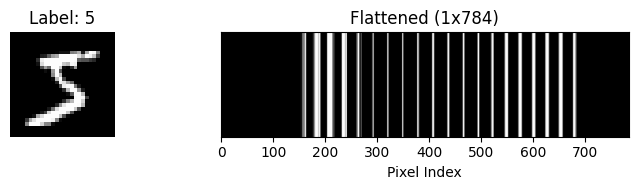
Flattened 28×28 images into 784-element vectors and fed them to fully-connected layers.
Noticed that the MLP treats every pixel independently — no spatial awareness.
Today we fix that with Convolutional Neural Networks.
# ── Setup ──────────────────────────────────────────────────────────────
import torch
import torch.nn as nn
import torch.nn.functional as F
import torch.optim as optim
from torch.utils.data import Dataset, DataLoader, TensorDataset

import torchvision
import torchvision.transforms as transforms

import numpy as np
import matplotlib.pyplot as plt

# For dropdown MCQs
from ipywidgets import Dropdown, VBox, HTML, Output
from IPython.display import display, clear_output

torch.manual_seed(42)
np.random.seed(42)

if torch.backends.mps.is_available():
    device = torch.device("mps")
elif torch.cuda.is_available():
    device = torch.device("cuda")
else:
    device = torch.device("cpu")

print(f"Using device: {device}")
Using device: mps
# ── MCQ Helper ─────────────────────────────────────────────────────────
# Creates a dropdown quiz question.  The answer is hidden until the
# student selects an option.

def mcq(question: str, options: dict, correct: str):
    """
    Display a multiple-choice question with a dropdown.

    Parameters
    ----------
    question : str
        The question text (supports HTML).
    options : dict
        Mapping of option labels to descriptions, e.g. {'A': 'Answer A', ...}
    correct : str
        The correct option label (e.g. 'B').
    """
    q_html = HTML(f"<h4 style='color:#2c3e50'>🤔 {question}</h4>")
    dropdown = Dropdown(
        options=['-- Select your answer --'] + [f'{k}) {v}' for k, v in options.items()],
        value='-- Select your answer --',
        description='Answer:',
        style={'description_width': 'initial'},
        layout={'width': '80%'}
    )
    feedback = Output()

    def on_change(change):
        if change['name'] == 'value' and change['new'] != '-- Select your answer --':
            selected = change['new'].split(')')[0]
            with feedback:
                clear_output()
                if selected == correct:
                    print(f'✅  Correct!  {correct}) {options[correct]}')
                else:
                    print(f'❌  Not quite. Try again!  (Hint: think about what makes CNNs special.)')

    dropdown.observe(on_change)
    display(VBox([q_html, dropdown, feedback]))
Part 1 — Why Do We Need CNNs? (~10 min)
The MLP Problem with Images
In Tutorial 5 we flattened each Fashion MNIST image into a 784-element vector and passed it through fully-connected (FC) layers. That approach has two serious problems when we scale up:
| Problem | What happens | Example |
|---|---|---|
| Parameter explosion | Every pixel connects to every neuron in the next layer. | A 256×256 RGB image → 196,608 inputs. With 1,000 hidden units that’s ~200 million weights — just for one layer! |
| No spatial awareness | The MLP sees pixels as unrelated numbers. | If you shift a cat 3 pixels to the right, the MLP sees a completely different input vector, even though it’s the same cat. |
Source
train_dataset = torchvision.datasets.MNIST(root='./data', train=True, download=True, transform=transforms.ToTensor())
# Take one image from the training set
image, label = train_dataset[0]

print("Original shape:", image.shape)  # Should be [1, 28, 28]

# Flatten the image to a 1D vector of length 784
flattened = image.view(-1)
print("Flattened shape:", flattened.shape)  # Should be [784]

# Optionally, show the first 20 values
print("First 20 pixel values:", flattened[:20])

import matplotlib.pyplot as plt

# Display the original image
plt.figure(figsize=(8, 2))

plt.subplot(1, 2, 1)
plt.imshow(image.squeeze(), cmap='gray')
plt.title(f"Label: {label}")
plt.axis('off')

# Display the flattened image as a row vector
plt.subplot(1, 2, 2)
plt.imshow(flattened.unsqueeze(0), cmap='gray', aspect='auto')
plt.title("Flattened (1x784)")
plt.xlabel("Pixel Index")
plt.yticks([])
plt.tight_layout()
plt.show()
Original shape: torch.Size([1, 28, 28])
Flattened shape: torch.Size([784])
First 20 pixel values: tensor([0., 0., 0., 0., 0., 0., 0., 0., 0., 0., 0., 0., 0., 0., 0., 0., 0., 0., 0., 0.])
Source
import torchvision.datasets as datasets
import torchvision.transforms as transforms
import matplotlib.pyplot as plt
import ipywidgets as widgets
from IPython.display import display, clear_output
import random

# 1. Download and load the MNIST dataset
print("Loading dataset... (this may take a moment if downloading for the first time)")
dataset = datasets.MNIST(root='./data', train=True, download=True, transform=transforms.ToTensor())
clear_output() # Clears the loading text once done

# 2. Global variables to store the current state
current_image = None
current_label = None

# 3. Create the UI widgets
out = widgets.Output()
guess_input = widgets.BoundedIntText(value=0, min=0, max=9, step=1, description='Guess:', layout=widgets.Layout(width='150px'))
submit_btn = widgets.Button(description='Submit Guess', button_style='success')
next_btn = widgets.Button(description='Load New Image', button_style='info')
feedback_label = widgets.HTML(value="<b>Click 'Load New Image' to begin!</b>")

# 4. Define button actions (callbacks)
def load_new_image(b):
    global current_image, current_label

    # Pick a random image
    idx = random.randint(0, len(dataset) - 1)
    current_image, current_label = dataset[idx]

    # Update UI for a new round
    feedback_label.value = "<b>Examine the 1D vector below. Enter your guess (0-9) and click Submit!</b>"

    with out:
        clear_output(wait=True)
        flattened = current_image.view(-1).unsqueeze(0)

        plt.figure(figsize=(10, 2))
        plt.imshow(flattened, cmap='gray', aspect='auto')
        plt.title("Mystery Flattened Image (1 x 784)")
        plt.xlabel("Pixel Index (0 to 783)")
        plt.yticks([])
        plt.show()

def submit_guess(b):
    global current_image, current_label
    if current_image is None:
        return

    guess = guess_input.value

    # Provide feedback
    if guess == current_label:
        feedback_label.value = f"<b style='color:green;'>Spot on!</b> You successfully decoded the matrix. It is a <b>{current_label}</b>."
    else:
        feedback_label.value = f"<b style='color:red;'>Not quite.</b> You guessed {guess}, but it was actually a <b>{current_label}</b>. This is why MLPs struggle!"

    # Reveal the original 2D image alongside the 1D vector
    with out:
        clear_output(wait=True)
        flattened = current_image.view(-1).unsqueeze(0)

        fig, axes = plt.subplots(2, 1, figsize=(10, 5))

        # Display Flattened
        axes[0].imshow(flattened, cmap='gray', aspect='auto')
        axes[0].set_title("What the MLP saw (Flattened 1D Vector)")
        axes[0].set_yticks([])

        # Display Original
        axes[1].imshow(current_image.squeeze(), cmap='gray')
        axes[1].set_title(f"What the CNN sees (Preserved 2D Topology)")
        axes[1].axis('off')

        plt.tight_layout()
        plt.show()

# 5. Connect buttons to actions
next_btn.on_click(load_new_image)
submit_btn.on_click(submit_guess)

# 6. Layout and display the UI
controls = widgets.HBox([guess_input, submit_btn, next_btn])
display(feedback_label, controls, out)The CNN Solution — Three Key Ideas
CNNs exploit the spatial structure of images with three elegant principles:
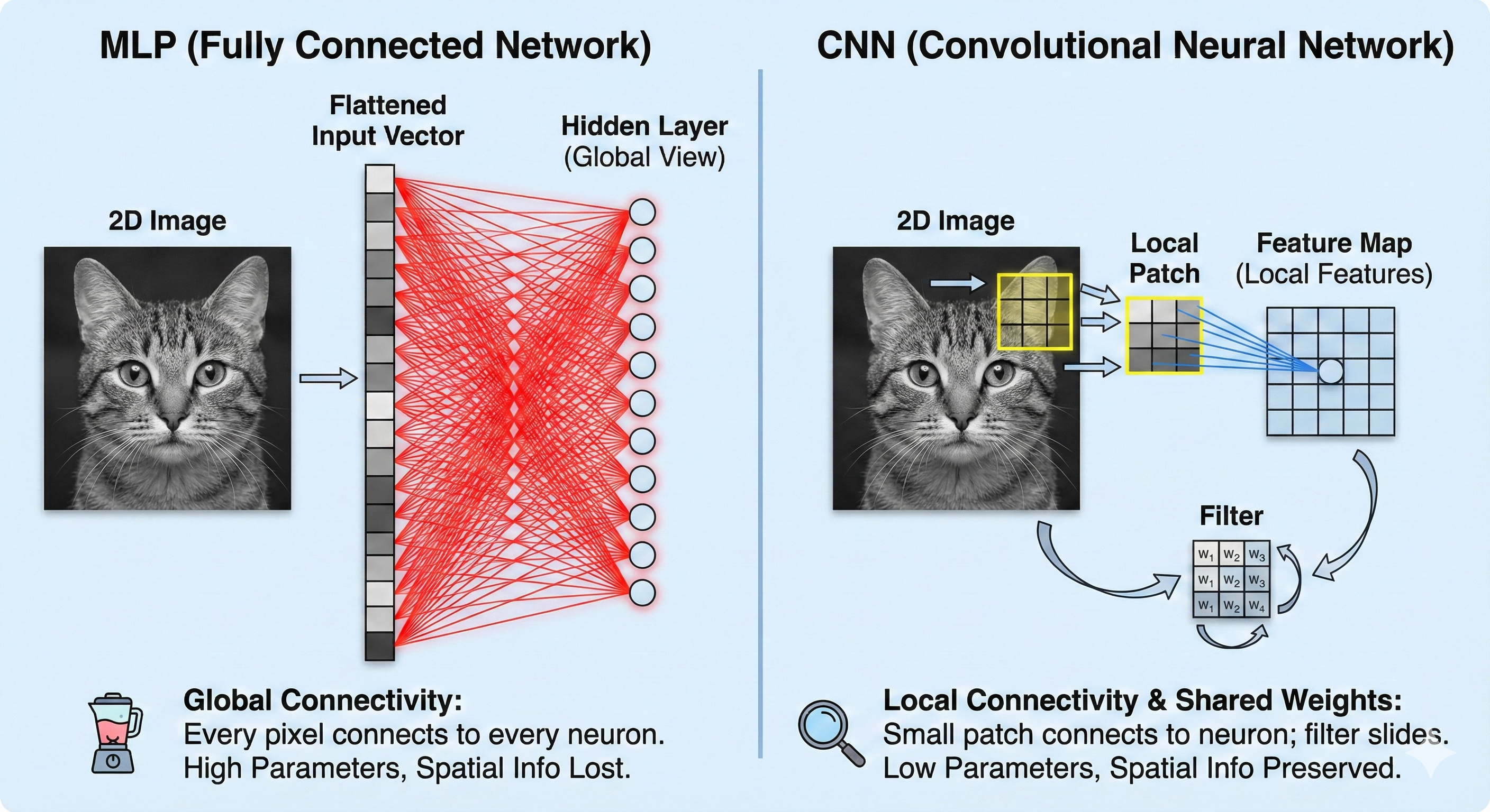
Local Connectivity (Receptive Fields)
Instead of connecting to every pixel, each neuron looks at a small patch of the image (e.g., 3×3 pixels). Nearby pixels are more related than distant ones.🔦 Analogy: Imagine shining a small flashlight on a mural. You can only see a small patch at a time, but by sliding the flashlight across the wall, you can examine the entire mural.
Weight Sharing (Filters/Kernels)
The same small set of weights (the filter) is reused as it slides across the image. This dramatically reduces parameters and lets the network detect a pattern anywhere in the image.🕵️ Analogy: Think of a “vertical-edge detector.” Whether the edge is in the top-left or bottom-right of the image, the same detector can find it.
Translation Invariance
Because the same filter scans everywhere, a CNN recognizes objects regardless of their position.🐱 A cat is a cat no matter where it sits in the picture.
Visual Comparison
Source
import torch
import torchvision.datasets as datasets
import torchvision.transforms as transforms
import matplotlib.pyplot as plt
import matplotlib.patches as patches
import ipywidgets as widgets
from IPython.display import display, clear_output
import random
import math

# 1. Load MNIST Dataset
print("Loading MNIST...")
dataset_mnist = datasets.MNIST(root='./data', train=True, download=True, transform=transforms.ToTensor())
clear_output()

# --- Helper Function for Spaced-Out Grayscale Patches ---
def get_spaced_mnist_patches(img_tensor, num_patches=3, patch_size=6):
    img_2d = img_tensor.squeeze()
    h, w = img_2d.shape
    patch_size = min(patch_size, h)

    if patch_size == h:
        return [img_2d.numpy()]*num_patches, [(0,0)]*num_patches, patch_size

    # 1. Calculate variance for all patches
    scored_patches = []
    for r in range(h - patch_size):
        for col in range(w - patch_size):
            patch = img_2d[r:r+patch_size, col:col+patch_size]
            variance = torch.var(patch).item()
            # Ignore completely blank/black areas to speed things up
            if variance > 0.01:
                scored_patches.append((variance, r, col))

    # Sort by variance (highest complexity first)
    scored_patches.sort(reverse=True, key=lambda x: x[0])

    # 2. Select patches with a distance constraint
    chosen = []
    # Require patches to be separated by at least 75% of the patch width, minimum 5 pixels
    min_dist = max(patch_size * 0.75, 5.0)

    for cand_var, cand_r, cand_c in scored_patches:
        too_close = False
        for _, chosen_r, chosen_c in chosen:
            # Euclidean distance formula
            dist = math.sqrt((cand_r - chosen_r)**2 + (cand_c - chosen_c)**2)
            if dist < min_dist:
                too_close = True
                break

        if not too_close:
            chosen.append((cand_var, cand_r, cand_c))

        if len(chosen) == num_patches:
            break

    # 3. Fallback (If the digit is too small to find 3 widely spaced patches)
    if len(chosen) < num_patches and len(scored_patches) > 0:
        top_pool = scored_patches[:max(1, len(scored_patches)//10)]
        for cand_var, cand_r, cand_c in top_pool:
            if (cand_var, cand_r, cand_c) not in chosen:
                chosen.append((cand_var, cand_r, cand_c))
            if len(chosen) == num_patches:
                break

    # Shuffle so the most complex patch isn't always the first one displayed
    random.shuffle(chosen)

    extracted_patches = []
    patch_coords = []

    for _, r, col in chosen:
        patch = img_2d[r:r+patch_size, col:col+patch_size]
        extracted_patches.append(patch.numpy())
        patch_coords.append((col, r))

    return extracted_patches, patch_coords, patch_size

# --- Game State & UI ---
current_image_mnist = None
current_label_mnist = None
current_coords_mnist = None
current_patch_size_mnist = None

out_mnist = widgets.Output()

patch_size_slider = widgets.IntSlider(
    value=6, min=2, max=28, step=2,
    description='Patch Size:',
    continuous_update=False,
    layout=widgets.Layout(width='300px')
)

guess_dropdown = widgets.Dropdown(options=list(range(10)), description='Guess Digit:')
submit_btn_mnist = widgets.Button(description='Submit Guess', button_style='success')
next_btn_mnist = widgets.Button(description='Load New Image', button_style='info')
feedback_label_mnist = widgets.HTML(value="<b>Adjust the patch size, guess the digit (0-9), and click Submit!</b>")

def load_new_mnist_round(b=None):
    global current_image_mnist, current_label_mnist, current_coords_mnist, current_patch_size_mnist

    is_new_image = (b is next_btn_mnist or current_image_mnist is None)

    if is_new_image:
        idx = random.randint(0, len(dataset_mnist) - 1)
        current_image_mnist, current_label_mnist = dataset_mnist[idx]
        feedback_label_mnist.value = "<b>Look at these distinct structural features. What digit do they form?</b>"

    p_size = patch_size_slider.value
    patches_list, coords, final_p_size = get_spaced_mnist_patches(current_image_mnist, num_patches=3, patch_size=p_size)
    current_coords_mnist = coords
    current_patch_size_mnist = final_p_size

    with out_mnist:
        clear_output(wait=True)
        fig, axes = plt.subplots(1, 3, figsize=(9, 3))
        for i, ax in enumerate(axes):
            if i < len(patches_list):
                ax.imshow(patches_list[i], cmap='gray', interpolation='nearest', vmin=0, vmax=1)
                ax.set_title(f"Receptive Field {i+1}\n({final_p_size}x{final_p_size})")

                if final_p_size <= 14:
                    import numpy as np
                    ax.set_xticks(np.arange(-.5, final_p_size, 1), minor=True)
                    ax.set_yticks(np.arange(-.5, final_p_size, 1), minor=True)
                    ax.grid(which='minor', color='red', linestyle='-', linewidth=0.5, alpha=0.3)
                    ax.tick_params(which='minor', bottom=False, left=False)

                ax.axis('off')
        plt.tight_layout()
        plt.show()

def submit_mnist_guess(b):
    global current_image_mnist, current_label_mnist, current_coords_mnist, current_patch_size_mnist
    if current_image_mnist is None: return

    guess = guess_dropdown.value

    if guess == current_label_mnist:
        feedback_label_mnist.value = f"<b style='color:green;'>Excellent!</b> You correctly synthesized the dispersed features to find the <b>{current_label_mnist}</b>."
    else:
        feedback_label_mnist.value = f"<b style='color:red;'>Not quite.</b> You guessed {guess}, but it was a <b>{current_label_mnist}</b>."

    with out_mnist:
        clear_output(wait=True)
        fig, ax = plt.subplots(figsize=(5, 5))
        ax.imshow(current_image_mnist.squeeze(), cmap='gray')
        ax.set_title(f"Original Image: {current_label_mnist}")

        if current_patch_size_mnist < 28:
            for (col, r) in current_coords_mnist:
                rect = patches.Rectangle((col - 0.5, r - 0.5),
                                         current_patch_size_mnist, current_patch_size_mnist,
                                         linewidth=2, edgecolor='red', facecolor='none')
                ax.add_patch(rect)

        ax.axis('off')
        plt.show()

next_btn_mnist.on_click(load_new_mnist_round)
submit_btn_mnist.on_click(submit_mnist_guess)
patch_size_slider.observe(lambda change: load_new_mnist_round(), names='value')

top_row = widgets.HBox([patch_size_slider, next_btn_mnist])
bottom_row = widgets.HBox([guess_dropdown, submit_btn_mnist])
ui_layout = widgets.VBox([top_row, bottom_row])

display(feedback_label_mnist, ui_layout, out_mnist)
load_new_mnist_round()✅ Check Your Understanding — MCQ Set 1
Q1: What is the MAIN reason CNNs use local connectivity instead of connecting every pixel to every neuron?
A) It makes the network deeper
B) Nearby pixels are more related, and it drastically reduces the number of parameters
C) It removes the need for activation functions
D) It requires more training data
Click to reveal solution
Answer: B) Nearby pixels are more related, and it drastically reduces the number of parameters
Q2: What does ‘weight sharing’ mean in the context of CNNs?
A) Each neuron has its own unique set of weights
B) The same filter (set of weights) is applied at every position across the image
C) Weights are shared between the training and test sets
D) All layers use the same weights
Click to reveal solution
Answer: B) The same filter (set of weights) is applied at every position across the image
Part 2 — The Convolution Operation: A Hands-On Demo (~15 min)
Let’s see convolution in action before we touch PyTorch. We’ll create a tiny 6×6 image and apply a 3×3 filter by hand (well, with NumPy).
What Is a Convolution (Cross-Correlation)?
Place the filter on the top-left corner of the image.
Multiply each filter value by the overlapping pixel value.
Sum all the products → this gives you one number in the output.
Slide the filter one step to the right (or down) and repeat.
The output grid is called a feature map.
Source
import numpy as np
import matplotlib.pyplot as plt

# --- Toy convolution demo ---

image = np.array([
    [0, 0, 0, 1, 1, 1],
    [0, 0, 0, 1, 1, 1],
    [0, 0, 0, 1, 1, 1],
    [0, 0, 0, 1, 1, 1],
    [0, 0, 0, 1, 1, 1],
    [0, 0, 0, 1, 1, 1],
], dtype=np.float32)

kernel = np.array([
    [-1, 0, 1],
    [-1, 0, 1],
    [-1, 0, 1],
], dtype=np.float32)

def convolve2d(img, kern):
    h, w = img.shape
    kh, kw = kern.shape
    out_h, out_w = h - kh + 1, w - kw + 1
    output = np.zeros((out_h, out_w))
    for i in range(out_h):
        for j in range(out_w):
            patch = img[i:i+kh, j:j+kw]
            output[i, j] = np.sum(patch * kern)
    return output

feature_map = convolve2d(image, kernel)

fig, axes = plt.subplots(1, 3, figsize=(16, 5))

# 1. Input Image with Pixel Values
axes[0].imshow(image, cmap='gray', vmin=0, vmax=1)
axes[0].set_title('Input Image (6×6)', fontsize=13, pad=15)
for i in range(image.shape[0]):
    for j in range(image.shape[1]):
        # Dynamic color: white text on dark pixels, black on light
        color = "white" if image[i, j] < 0.5 else "black"
        axes[0].text(j, i, f'{image[i,j]:.0f}', ha='center', va='center',
                     fontsize=12, fontweight='bold', color=color)
axes[0].axis('off')

# 2. Filter / Kernel
axes[1].imshow(kernel, cmap='RdBu', vmin=-1, vmax=1)
axes[1].set_title('Filter / Kernel (3×3)', fontsize=13, pad=15)
for i in range(3):
    for j in range(3):
        axes[1].text(j, i, f'{kernel[i,j]:.0f}', ha='center', va='center',
                     fontsize=14, fontweight='bold')
axes[1].axis('off')

# 3. Feature Map
axes[2].imshow(feature_map, cmap='hot')
axes[2].set_title('Feature Map (4×4)', fontsize=13, pad=15)
for i in range(feature_map.shape[0]):
    for j in range(feature_map.shape[1]):
        axes[2].text(j, i, f'{feature_map[i,j]:.0f}', ha='center', va='center',
                     fontsize=14, fontweight='bold', color='cyan')
axes[2].axis('off')

plt.suptitle('Convolution in Action: Detecting a Vertical Edge', fontsize=16, fontweight='bold', y=1.05)
plt.tight_layout()
plt.show()

print('\n📝 Analysis:')
print(f'   The maximum value in the feature map is {np.max(feature_map):.0f}.')
print('   This occurs because the 3x3 kernel aligns perfectly with the 0-to-1 transition.')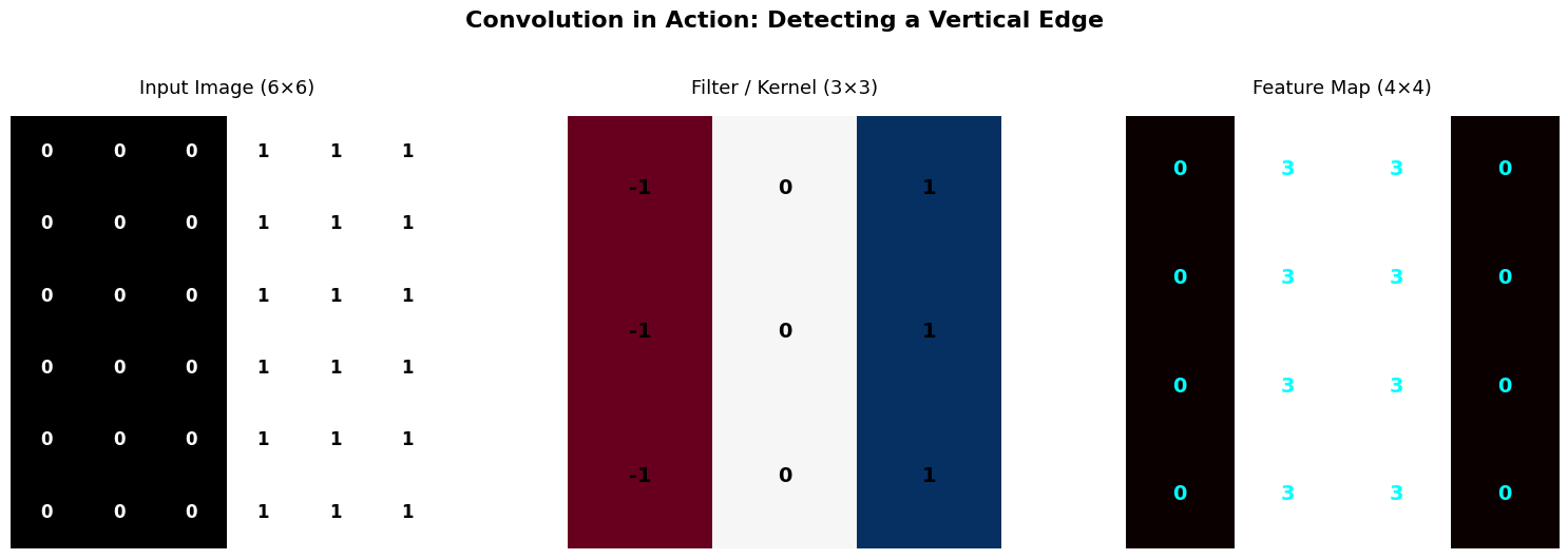
📝 Analysis:
   The maximum value in the feature map is 3.
   This occurs because the 3x3 kernel aligns perfectly with the 0-to-1 transition.
🧮 Trace It Yourself!
Let’s manually compute one element of the feature map. Place the kernel at position (0, 0):
Image patch:          Filter:
  0  0  0               -1  0  1
  0  0  0       ×       -1  0  1
  0  0  0               -1  0  1

Element-wise multiply:  0  0  0
                        0  0  0
                        0  0  0

Sum = 0
Now try position (0, 2) — right at the edge:
Image patch:          Filter:
  0  1  1               -1  0  1
  0  1  1       ×       -1  0  1
  0  1  1               -1  0  1

Element-wise:    0  0  1
                 0  0  1
                 0  0  1

Sum = 3  ← The edge is detected!
Key Insight: The filter doesn’t know where the edge is ahead of time — it discovers it by sliding across the image. This is the power of convolution!
Source
import numpy as np
import plotly.graph_objects as go
from plotly.subplots import make_subplots

# --- 1. Define the Data ---
image = np.array([
    [0, 0, 0, 1, 1, 1],
    [0, 0, 0, 1, 1, 1],
    [0, 0, 0, 1, 1, 1],
    [0, 0, 0, 1, 1, 1],
    [0, 0, 0, 1, 1, 1],
    [0, 0, 0, 1, 1, 1],
], dtype=np.float32)

kernel = np.array([
    [-1, 0, 1],
    [-1, 0, 1],
    [-1, 0, 1],
], dtype=np.float32)

h, w = image.shape
kh, kw = kernel.shape
out_h, out_w = h - kh + 1, w - kw + 1

# Pre-calculate the full feature map
full_feature_map = np.zeros((out_h, out_w))
for i in range(out_h):
    for j in range(out_w):
        full_feature_map[i, j] = np.sum(image[i:i+kh, j:j+kw] * kernel)

# --- 2. Setup Figure and Base Traces ---
fig = make_subplots(rows=1, cols=2, horizontal_spacing=0.1,
                    subplot_titles=("Input Image (6x6)", "Feature Map (Accumulating)"))

# Trace 0: Input Image Heatmap
fig.add_trace(go.Heatmap(z=image, colorscale='gray', showscale=False, zmin=0, zmax=1, hoverinfo='skip'), row=1, col=1)

# Trace 1: Input Image Text Overlay
img_y, img_x = np.mgrid[0:h, 0:w]
img_text = [f"{val:.0f}" for val in image.flatten()]
img_colors = ['white' if val < 0.5 else 'black' for val in image.flatten()]
fig.add_trace(go.Scatter(
    x=img_x.flatten(), y=img_y.flatten(), mode='text', text=img_text,
    textfont=dict(color=img_colors, size=14, family="Arial"), hoverinfo='skip'
), row=1, col=1)

# Trace 2: Feature Map Heatmap (Starts with NaNs so it's empty)
init_fm = np.full((out_h, out_w), np.nan)
fig.add_trace(go.Heatmap(z=init_fm, colorscale='hot', showscale=False, zmin=-3, zmax=3, hoverinfo='skip'), row=1, col=2)

# Trace 3: Feature Map Text Overlay (Starts empty)
fm_y, fm_x = np.mgrid[0:out_h, 0:out_w]
fig.add_trace(go.Scatter(
    x=fm_x.flatten(), y=fm_y.flatten(), mode='text', text=['']*(out_h*out_w),
    textfont=dict(color='cyan', size=14, family="Arial Black"), hoverinfo='skip'
), row=1, col=2)

# Trace 4: Sliding Window Bounding Box (Green Square)
fig.add_trace(go.Scatter(
    x=[-0.5, 2.5, 2.5, -0.5, -0.5], y=[-0.5, -0.5, 2.5, 2.5, -0.5],
    mode='lines', line=dict(color='lime', width=4), hoverinfo='skip'
), row=1, col=1)

# --- 3. Create Animation Frames ---
frames = []
steps = []

for step_idx in range(out_h * out_w):
    y_pos = step_idx // out_w
    x_pos = step_idx % out_w

    # Build the feature map state up to the current step
    curr_fm = np.full((out_h, out_w), np.nan)
    curr_text = [''] * (out_h * out_w)

    for k in range(step_idx + 1):
        r, c = k // out_w, k % out_w
        curr_fm[r, c] = full_feature_map[r, c]
        curr_text[k] = f"{full_feature_map[r, c]:.0f}"

    # Move the bounding box
    x_box = [x_pos - 0.5, x_pos + 2.5, x_pos + 2.5, x_pos - 0.5, x_pos - 0.5]
    y_box = [y_pos - 0.5, y_pos - 0.5, y_pos + 2.5, y_pos + 2.5, y_pos - 0.5]

    # Assign updates only to Traces 2, 3, and 4
    frame = go.Frame(
        name=str(step_idx),
        data=[
            go.Heatmap(z=curr_fm),      # Updates Feature Map colors
            go.Scatter(text=curr_text), # Updates Feature Map text
            go.Scatter(x=x_box, y=y_box)# Updates Bounding Box position
        ],
        traces=[2, 3, 4]
    )
    frames.append(frame)

    # Link the frame to a step on the slider
    step_dict = dict(
        method="animate",
        args=[[str(step_idx)], {"frame": {"duration": 0, "redraw": True}, "mode": "immediate", "transition": {"duration": 0}}],
        label=f"Row {y_pos}, Col {x_pos}"
    )
    steps.append(step_dict)

fig.frames = frames

# --- 4. Layout and Styling ---
fig.update_layout(
    width=900, height=500, plot_bgcolor='white', showlegend=False,
    sliders=[dict(active=0, currentvalue={"prefix": "Current Step: "}, pad={"t": 40}, steps=steps)]
)

# Fix axes so they behave like images (inverted Y-axis, square pixels, hide gridlines)
fig.update_xaxes(showticklabels=False, showgrid=False, zeroline=False, scaleanchor="y", scaleratio=1)
fig.update_yaxes(showticklabels=False, showgrid=False, zeroline=False, autorange="reversed")

fig.show()✅ Check Your Understanding — MCQ Set 2
Q3: What does a convolutional filter (kernel) detect in an image?
A) It transforms every pixel independently, like a lookup table
B) It detects a specific local pattern (like edges, corners, or textures)
C) It fills in missing pixel values
D) It always increases the size of the image
Click to reveal solution
Answer: B) It detects a specific local pattern (like edges, corners, or textures)
Q4: If we apply a 3×3 filter (stride=1, no padding) to a 6×6 image, what is the size of the output feature map?
A) 6×6
B) 3×3
C) 4×4
D) 5×5
Click to reveal solution
Answer: C) 4×4
Part 3 — Key CNN Building Blocks (~10 min)
A CNN is built from a few simple components stacked together:
3.1 Convolutional Layer
Applies multiple filters to the input.
Each filter produces one feature map.
If we use 16 filters, we get 16 feature maps — the network learns 16 different patterns.
Key parameters:
kernel_size: How big the filter is (e.g., 3×3)stride: How far the filter moves each step (usually 1)padding: Zero-pixels added around the border to control output size
Output size formula:
from IPython.display import IFrame, display

display(IFrame(
    src="https://poloclub.github.io/cnn-explainer/?norec=true",
    width="100%",
    height=400
))1. Padding
Padding involves adding extra pixels (usually zeros) around the edges of an input map.
Data Preservation: It prevents the loss of information at the borders of the activation map.
Spatial Size: It allows the output to maintain the same dimensions as the input, enabling the construction of deeper networks.
Zero-Padding: This is the industry standard due to its simplicity, efficiency, and proven success in models like AlexNet.
2. Kernel Size (Filter Size)
The kernel is the “sliding window” that extracts features from the input.
Small Kernels (e.g., 3x3):
Extract highly local, detailed features.
Cause a slower reduction in layer dimensions, allowing for more layers (depth).
Generally lead to better performance in image classification by learning complex features.
Large Kernels:
Extract broader, larger features.
Lead to a rapid reduction in dimensions, which often limits network depth and performance.
3. Stride
Stride defines the “step size” of the kernel as it moves across the input.
Low Stride (e.g., 1): The kernel moves one pixel at a time, capturing more data and resulting in larger output layers.
High Stride: The kernel jumps more pixels, resulting in faster dimensionality reduction and less granular feature extraction.
Symmetry: Designers must ensure the stride allows the kernel to move symmetrically across the input without “hanging off” the edge unevenly.
3.2 Activation Function (ReLU)
Same ReLU you already know:
Introduces non-linearity — without it, stacking conv layers would just be a fancy linear transformation.
3.3 Pooling Layer
Shrinks the spatial dimensions (height & width) while keeping the most important information.
Makes the network robust to small shifts in the input.
Two common types:
Max Pooling — keeps the largest value in each window (most popular).
Average Pooling — keeps the average value in each window.
Pooling Demo
Source
# ── Pooling visualization ─────────────────────────────────────────────
feature = np.array([
    [1, 3, 2, 4],
    [5, 6, 1, 2],
    [7, 2, 3, 1],
    [0, 8, 4, 5],
], dtype=np.float32)

# 2×2 Max Pooling
max_pool = np.array([
    [max(feature[0,0], feature[0,1], feature[1,0], feature[1,1]),
     max(feature[0,2], feature[0,3], feature[1,2], feature[1,3])],
    [max(feature[2,0], feature[2,1], feature[3,0], feature[3,1]),
     max(feature[2,2], feature[2,3], feature[3,2], feature[3,3])],
])

# 2×2 Average Pooling
avg_pool = np.array([
    [np.mean(feature[0:2, 0:2]), np.mean(feature[0:2, 2:4])],
    [np.mean(feature[2:4, 0:2]), np.mean(feature[2:4, 2:4])],
])

fig, axes = plt.subplots(1, 3, figsize=(14, 4))
for ax, data, title in zip(axes, [feature, max_pool, avg_pool],
                            ['Feature Map (4×4)', 'Max Pool 2×2 → (2×2)', 'Avg Pool 2×2 → (2×2)']):
    ax.imshow(data, cmap='YlOrRd', vmin=0, vmax=8)
    for i in range(data.shape[0]):
        for j in range(data.shape[1]):
            ax.text(j, i, f'{data[i,j]:.1f}', ha='center', va='center', fontsize=16, fontweight='bold')
    ax.set_title(title, fontsize=13)
    ax.axis('off')
plt.suptitle('Pooling Operations Illustrated', fontsize=15, fontweight='bold')
plt.tight_layout()
plt.show()

print('Max pooling keeps the STRONGEST response in each 2×2 window.')
print('Average pooling smooths things out — useful in some architectures.')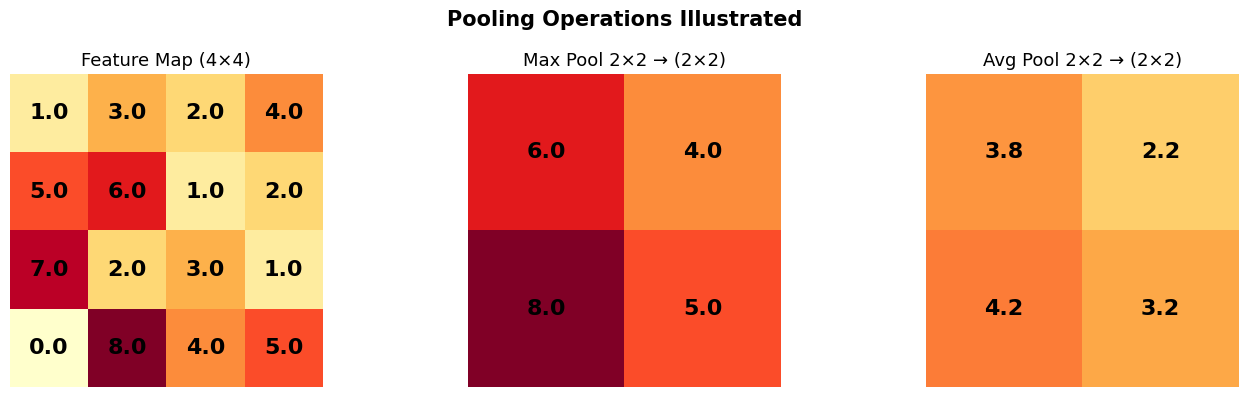
Max pooling keeps the STRONGEST response in each 2×2 window.
Average pooling smooths things out — useful in some architectures.
3.4 Fully-Connected (FC) Layer
After extracting features with conv + pool layers, we flatten the feature maps into a vector.
This vector goes through one or more FC layers (just like the MLPs in Tutorial 5) to produce the final class predictions.
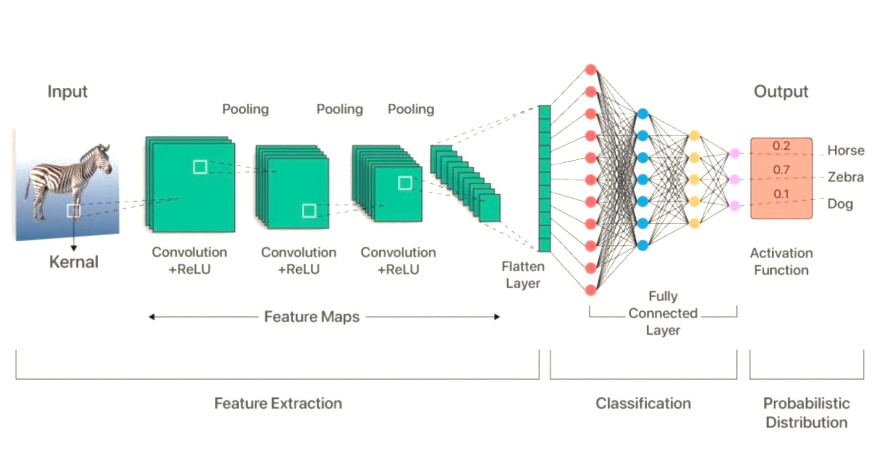
The Typical CNN Pipeline
✅ Check Your Understanding — MCQ Set 3
Q5: Why do we apply pooling after a convolution?
A) To increase the spatial resolution of the feature maps
B) To reduce spatial dimensions and make the network robust to small shifts
C) To add more learnable parameters
D) To disable the activation function
Click to reveal solution
Answer: B) To reduce spatial dimensions and make the network robust to small shifts
Q6: In simple terms, what does a feature map represent?
A) A single pixel value from the original image
B) The response of one filter applied across the entire image
C) The ground truth labels
D) The learning rate schedule
Click to reveal solution
Answer: B) The response of one filter applied across the entire image
Part 4 — Your First CNN: A Toy Synthetic Dataset (~15 min)
Before jumping to a real dataset, let’s build intuition with a tiny problem.
Task: Classify 8×8 grayscale images into two classes:
Class 0: Has a bright vertical stripe in the center
Class 1: Has a bright horizontal stripe in the center
This is dead simple for a CNN (it just needs an edge detector!) but will let us see every moving part.
Source
# ── Synthetic stripe dataset ──────────────────────────────────────────

def make_stripe_data(n_samples=400, img_size=8):
    """Create a tiny dataset of vertical vs horizontal stripes."""
    images = []
    labels = []
    for i in range(n_samples):
        # Start with random noise
        img = np.random.randn(img_size, img_size).astype(np.float32) * 0.2
        if i % 2 == 0:
            # Class 0: vertical stripe (columns 3-4 are bright)
            img[:, 3:5] += 1.0
            labels.append(0)
        else:
            # Class 1: horizontal stripe (rows 3-4 are bright)
            img[3:5, :] += 1.0
            labels.append(1)
        images.append(img)

    X = torch.tensor(np.array(images)).unsqueeze(1)  # (N, 1, 8, 8)
    y = torch.tensor(labels)
    return X, y

X_toy, y_toy = make_stripe_data(400)

# Train/test split
X_train_toy, X_test_toy = X_toy[:320], X_toy[320:]
y_train_toy, y_test_toy = y_toy[:320], y_toy[320:]

train_toy_loader = DataLoader(TensorDataset(X_train_toy, y_train_toy), batch_size=32, shuffle=True)
test_toy_loader  = DataLoader(TensorDataset(X_test_toy, y_test_toy), batch_size=32)

# Visualize a few samples
fig, axes = plt.subplots(2, 5, figsize=(12, 5))
for i, ax in enumerate(axes[0]):
    ax.imshow(X_train_toy[i*2, 0], cmap='gray')
    ax.set_title(f'Class 0 (vertical)', fontsize=10)
    ax.axis('off')
for i, ax in enumerate(axes[1]):
    ax.imshow(X_train_toy[i*2+1, 0], cmap='gray')
    ax.set_title(f'Class 1 (horizontal)', fontsize=10)
    ax.axis('off')
plt.suptitle('Toy Dataset: Vertical vs Horizontal Stripes', fontsize=14, fontweight='bold')
plt.tight_layout()
plt.show()

print(f'Training samples: {len(X_train_toy)}, Test samples: {len(X_test_toy)}')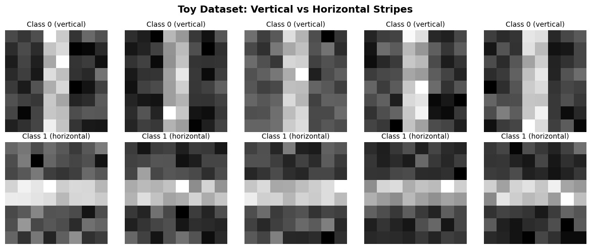
Training samples: 320, Test samples: 80
4.1 Building the Toy CNN
class TinyCNN(nn.Module):
    """
    A minimal CNN for 8×8 grayscale images.

    Architecture:
        Conv2d(1→4, 3×3, pad=1)  →  ReLU  →  MaxPool(2×2)  →  Flatten  →  FC(64→2)

    Shape walkthrough:
        Input:    (batch, 1,  8, 8)
        Conv:     (batch, 4,  8, 8)   ← padding=1 keeps size
        ReLU:     (batch, 4,  8, 8)
        MaxPool:  (batch, 4,  4, 4)   ← 8/2 = 4
        Flatten:  (batch, 4*4*4) = (batch, 64)
        FC:       (batch, 2)
    """
    def __init__(self):
        super().__init__()
        self.conv1 = nn.Conv2d(in_channels=1, out_channels=4, kernel_size=3, padding=1)
        self.pool  = nn.MaxPool2d(kernel_size=2, stride=2)
        self.fc1   = nn.Linear(4 * 4 * 4, 2)  # 4 channels × 4 height × 4 width

    def forward(self, x):
        x = self.pool(F.relu(self.conv1(x)))   # (batch, 4, 4, 4)
        x = x.view(x.size(0), -1)              # flatten
        x = self.fc1(x)
        return x

toy_model = TinyCNN().to(device)
print(toy_model)
print(f'\nTotal parameters: {sum(p.numel() for p in toy_model.parameters()):,}')
TinyCNN(
(conv1): Conv2d(1, 4, kernel_size=(3, 3), stride=(1, 1), padding=(1, 1))
(pool): MaxPool2d(kernel_size=2, stride=2, padding=0, dilation=1, ceil_mode=False)
(fc1): Linear(in_features=64, out_features=2, bias=True)
)
Total parameters: 170
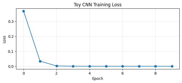
4.2 Training the Toy CNN
Notice how few epochs it takes — the problem is easy, and the CNN finds the right pattern quickly.
# ── Train the toy CNN ─────────────────────────────────────────────────
criterion = nn.CrossEntropyLoss()
optimizer = optim.Adam(toy_model.parameters(), lr=0.01)

toy_losses = []
for epoch in range(10):
    toy_model.train()
    epoch_loss = 0.0
    for xb, yb in train_toy_loader:
        xb, yb = xb.to(device), yb.to(device)
        out = toy_model(xb)
        loss = criterion(out, yb)
        optimizer.zero_grad()
        loss.backward()
        optimizer.step()
        epoch_loss += loss.item()
    avg_loss = epoch_loss / len(train_toy_loader)
    toy_losses.append(avg_loss)
    if (epoch + 1) % 2 == 0:
        print(f'Epoch {epoch+1:2d}/10  Loss: {avg_loss:.4f}')

# Plot the loss
plt.figure(figsize=(8, 3))
plt.plot(toy_losses, marker='o')
plt.title('Toy CNN Training Loss')
plt.xlabel('Epoch')
plt.ylabel('Loss')
plt.grid(True, alpha=0.3)
plt.show()
Epoch 2/10 Loss: 0.0341
Epoch 4/10 Loss: 0.0006
Epoch 6/10 Loss: 0.0002
Epoch 8/10 Loss: 0.0002
Epoch 10/10 Loss: 0.0002
# ── Evaluate on toy test set ──────────────────────────────────────────
toy_model.eval()
correct = 0
total = 0
with torch.no_grad():
    for xb, yb in test_toy_loader:
        xb, yb = xb.to(device), yb.to(device)
        preds = toy_model(xb).argmax(dim=1)
        correct += (preds == yb).sum().item()
        total += yb.size(0)

print(f'\n🎯 Toy CNN Test Accuracy: {100.0 * correct / total:.1f}%')
print('  (Should be near 100% — this is an easy task for a CNN!)')
🎯 Toy CNN Test Accuracy: 100.0%
  (Should be near 100% — this is an easy task for a CNN!)
4.3 What Did the Filters Learn?
Let’s peek at the 4 learned filters. Since our task is about vertical vs horizontal stripes, we’d expect some filters to respond to vertical patterns and others to horizontal patterns.
# ── Visualize learned filters ─────────────────────────────────────────
filters = toy_model.conv1.weight.detach().cpu().numpy()  # (4, 1, 3, 3)

fig, axes = plt.subplots(1, 4, figsize=(12, 3))
for i, ax in enumerate(axes):
    k = filters[i, 0]  # (3, 3)
    im = ax.imshow(k, cmap='RdBu', vmin=-k.max(), vmax=k.max())
    for r in range(3):
        for c in range(3):
            ax.text(c, r, f'{k[r,c]:.2f}', ha='center', va='center', fontsize=10)
    ax.set_title(f'Filter {i}', fontsize=12)
    ax.axis('off')
plt.suptitle('Learned Filters from Toy CNN', fontsize=14, fontweight='bold')
plt.tight_layout()
plt.show()

print('🔍 Look for patterns: do any filters resemble vertical or horizontal edge detectors?')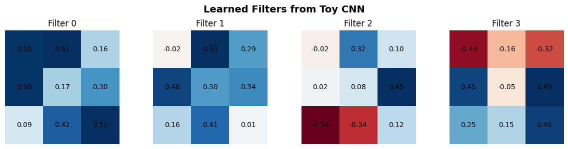
🔍 Look for patterns: do any filters resemble vertical or horizontal edge detectors?
✅ Check Your Understanding — MCQ Set 4
Q7: If a CNN uses 3×3 filters with stride 1 and padding 1, how does the output spatial size compare to the input?
A) It stays the same (same height and width)
B) It becomes larger
C) It becomes half the size
D) It depends on the number of filters
Click to reveal solution
Answer: A) It stays the same (same height and width)
Q8: If you shift an object slightly in an image, a well-trained CNN’s prediction should:
A) Change wildly every time
B) Stay relatively stable (translation invariance!)
C) Always become incorrect
D) Depend only on the color of the object
Click to reveal solution
Answer: B) Stay relatively stable (translation invariance!)
Part 5 — Scaling Up: CNN on CIFAR-10 (~20 min)
Now let’s tackle a real image classification task.
About CIFAR-10
60,000 color images (32×32 pixels, 3 color channels: RGB)
10 classes: airplane, automobile, bird, cat, deer, dog, frog, horse, ship, truck
50,000 training images, 10,000 test images
A classic benchmark — easy enough to train on a laptop, hard enough to be interesting.
# ── Load CIFAR-10 ─────────────────────────────────────────────────────
classes = ('airplane', 'automobile', 'bird', 'cat', 'deer',
           'dog', 'frog', 'horse', 'ship', 'truck')

# Simple transforms — we'll add augmentation later
transform_train = transforms.Compose([
    transforms.RandomHorizontalFlip(),  # simple augmentation
    transforms.ToTensor(),
    transforms.Normalize((0.5, 0.5, 0.5), (0.5, 0.5, 0.5))  # scale to [-1, 1]
])

transform_test = transforms.Compose([
    transforms.ToTensor(),
    transforms.Normalize((0.5, 0.5, 0.5), (0.5, 0.5, 0.5))
])

train_dataset = torchvision.datasets.CIFAR10(
    root='./data', train=True, download=True, transform=transform_train
)
test_dataset = torchvision.datasets.CIFAR10(
    root='./data', train=False, download=True, transform=transform_test
)

batch_size = 64
train_loader = DataLoader(train_dataset, batch_size=batch_size, shuffle=True)
test_loader  = DataLoader(test_dataset, batch_size=batch_size, shuffle=False)

print(f'Training samples: {len(train_dataset):,}')
print(f'Test samples:     {len(test_dataset):,}')
print(f'Image shape:      {train_dataset[0][0].shape}  (C, H, W)')
Training samples: 50,000
Test samples: 10,000
Image shape: torch.Size([3, 32, 32]) (C, H, W)
# ── Visualize some CIFAR-10 samples ───────────────────────────────────
def imshow(img, title=None):
    img = img / 2 + 0.5  # unnormalize from [-1,1] to [0,1]
    plt.figure(figsize=(12, 3))
    plt.imshow(np.transpose(img.numpy(), (1, 2, 0)))
    if title:
        plt.title(title, fontsize=13)
    plt.axis('off')
    plt.show()

dataiter = iter(train_loader)
images, labels = next(dataiter)

imshow(torchvision.utils.make_grid(images[:8]),
       title='  |  '.join(classes[l] for l in labels[:8]))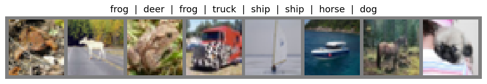
5.1 SimpleCNN — Our First Real Model
We start with a simple two-layer CNN. The architecture:
Conv(3→16, 3×3, pad=1) → ReLU → MaxPool(2×2)    # 32→16
Conv(16→32, 3×3, pad=1) → ReLU → MaxPool(2×2)   # 16→8
Flatten → FC(32*8*8 → 128) → ReLU → FC(128 → 10)
class SimpleCNN(nn.Module):
def __init__(self):
super().__init__()
# Convolutional feature extractor
self.conv1 = nn.Conv2d(3, 16, kernel_size=3, padding=1) # 3 input channels (RGB) → 16 filters
self.conv2 = nn.Conv2d(16, 32, kernel_size=3, padding=1) # 16 → 32 filters
self.pool = nn.MaxPool2d(2, 2) # halves spatial dims
# Classifier
self.fc1 = nn.Linear(32 * 8 * 8, 128) # 32 channels × 8×8 spatial
self.fc2 = nn.Linear(128, 10) # 10 classes
def forward(self, x):
# x: (batch, 3, 32, 32)
x = self.pool(F.relu(self.conv1(x))) # → (batch, 16, 16, 16)
x = self.pool(F.relu(self.conv2(x))) # → (batch, 32, 8, 8)
x = x.view(-1, 32 * 8 * 8) # flatten
x = F.relu(self.fc1(x)) # → (batch, 128)
x = self.fc2(x) # → (batch, 10)
return x
simple_model = SimpleCNN().to(device)
print(simple_model)
print(f'\nTotal parameters: {sum(p.numel() for p in simple_model.parameters()):,}')SimpleCNN(
(conv1): Conv2d(3, 16, kernel_size=(3, 3), stride=(1, 1), padding=(1, 1))
(conv2): Conv2d(16, 32, kernel_size=(3, 3), stride=(1, 1), padding=(1, 1))
(pool): MaxPool2d(kernel_size=2, stride=2, padding=0, dilation=1, ceil_mode=False)
(fc1): Linear(in_features=2048, out_features=128, bias=True)
(fc2): Linear(in_features=128, out_features=10, bias=True)
)
Total parameters: 268,650
5.2 Training the SimpleCNN
# ── Reusable training function ────────────────────────────────────────

def train_and_evaluate(model, train_loader, test_loader, num_epochs=10, lr=0.001):
    """Train a model and return loss history + final accuracy."""
    criterion = nn.CrossEntropyLoss()
    optimizer = optim.Adam(model.parameters(), lr=lr)

    train_losses = []

    for epoch in range(num_epochs):
        model.train()
        running_loss = 0.0
        for i, (images, labels) in enumerate(train_loader):
            images, labels = images.to(device), labels.to(device)

            outputs = model(images)
            loss = criterion(outputs, labels)

            optimizer.zero_grad()
            loss.backward()
            optimizer.step()

            running_loss += loss.item()

        avg_loss = running_loss / len(train_loader)
        train_losses.append(avg_loss)

        # Quick accuracy check every 2 epochs
        if (epoch + 1) % 2 == 0 or epoch == 0:
            model.eval()
            correct, total = 0, 0
            with torch.no_grad():
                for images, labels in test_loader:
                    images, labels = images.to(device), labels.to(device)
                    preds = model(images).argmax(1)
                    correct += (preds == labels).sum().item()
                    total += labels.size(0)
            print(f'Epoch {epoch+1:2d}/{num_epochs}  Loss: {avg_loss:.4f}  '
                  f'Test Acc: {100*correct/total:.1f}%')

    # Final accuracy
    model.eval()
    correct, total = 0, 0
    with torch.no_grad():
        for images, labels in test_loader:
            images, labels = images.to(device), labels.to(device)
            preds = model(images).argmax(1)
            correct += (preds == labels).sum().item()
            total += labels.size(0)
    final_acc = 100 * correct / total
    print(f'\n🎯 Final Test Accuracy: {final_acc:.2f}%')

    return train_losses, final_acc
print('Training SimpleCNN on CIFAR-10...')
print('=' * 50)
simple_losses, simple_acc = train_and_evaluate(
simple_model, train_loader, test_loader, num_epochs=10, lr=0.001
)Training SimpleCNN on CIFAR-10...
==================================================
Epoch 1/10 Loss: 1.4471 Test Acc: 56.6%
Epoch 2/10 Loss: 1.1223 Test Acc: 62.0%
Epoch 4/10 Loss: 0.8976 Test Acc: 67.0%
Epoch 6/10 Loss: 0.7809 Test Acc: 70.3%
Epoch 8/10 Loss: 0.6986 Test Acc: 70.8%
Epoch 10/10 Loss: 0.6318 Test Acc: 72.4%
🎯 Final Test Accuracy: 72.40%
✅ Check Your Understanding — MCQ Set 5
Q9: In our SimpleCNN, the first Conv2d layer has parameters Conv2d(3, 16, 3, padding=1). What does the ‘3’ as the first argument represent?
A) The kernel size (3×3)
B) The number of input channels (RGB = 3)
C) The stride value
D) The number of output classes
Click to reveal solution
Answer: B) The number of input channels (RGB = 3)
Q10: After two MaxPool2d(2,2) operations on a 32×32 input, what is the spatial size?
A) 16×16
B) 4×4
C) 8×8
D) 32×32 (unchanged)
Click to reveal solution
Answer: C) 8×8
Part 6 — Making It Better: BatchNorm, Dropout & Deeper Networks (~15 min)
Our SimpleCNN works, but we can do better with two common techniques:
Batch Normalization
What it does: Normalizes the output of each layer to have ~zero mean and ~unit variance during training.
Why it helps: Stabilizes training, allows higher learning rates, and acts as a mild regularizer.
Analogy: Imagine everyone in class takes an exam, but some questions are scored 0–10 and others 0–1000. BatchNorm “rescales” everything to a comparable range so learning is smoother.
Dropout
What it does: During training, randomly “turns off” a fraction of neurons (sets them to 0).
Why it helps: Prevents the network from relying too heavily on any single neuron — forces it to learn redundant, robust features.
Analogy: Imagine a group project where random team members call in sick each day. The team learns to distribute knowledge so no single person is a bottleneck.
class ImprovedCNN(nn.Module):
    """
    A deeper CNN with BatchNorm and Dropout.

    Architecture:
        Block 1: Conv(3→32) → BN → ReLU → Conv(32→32) → BN → ReLU → MaxPool → Dropout
        Block 2: Conv(32→64) → BN → ReLU → Conv(64→64) → BN → ReLU → MaxPool → Dropout
        Classifier: FC(64*8*8 → 256) → BN → ReLU → Dropout → FC(256 → 10)
    """
    def __init__(self):
        super().__init__()
        # Block 1
        self.conv1 = nn.Conv2d(3, 32, 3, padding=1)
        self.bn1   = nn.BatchNorm2d(32)
        self.conv2 = nn.Conv2d(32, 32, 3, padding=1)
        self.bn2   = nn.BatchNorm2d(32)

        # Block 2
        self.conv3 = nn.Conv2d(32, 64, 3, padding=1)
        self.bn3   = nn.BatchNorm2d(64)
        self.conv4 = nn.Conv2d(64, 64, 3, padding=1)
        self.bn4   = nn.BatchNorm2d(64)

        self.pool    = nn.MaxPool2d(2, 2)
        self.dropout = nn.Dropout(0.25)

        # Classifier
        self.fc1 = nn.Linear(64 * 8 * 8, 256)
        self.bn5 = nn.BatchNorm1d(256)
        self.fc2 = nn.Linear(256, 10)

    def forward(self, x):
        # Block 1: 32×32 → 16×16
        x = F.relu(self.bn1(self.conv1(x)))
        x = self.pool(F.relu(self.bn2(self.conv2(x))))
        x = self.dropout(x)

        # Block 2: 16×16 → 8×8
        x = F.relu(self.bn3(self.conv3(x)))
        x = self.pool(F.relu(self.bn4(self.conv4(x))))
        x = self.dropout(x)

        # Classifier
        x = x.view(-1, 64 * 8 * 8)
        x = F.relu(self.bn5(self.fc1(x)))
        x = self.dropout(x)
        x = self.fc2(x)
        return x

improved_model = ImprovedCNN().to(device)
print(improved_model)
print(f'\nTotal parameters: {sum(p.numel() for p in improved_model.parameters()):,}')
ImprovedCNN(
(conv1): Conv2d(3, 32, kernel_size=(3, 3), stride=(1, 1), padding=(1, 1))
(bn1): BatchNorm2d(32, eps=1e-05, momentum=0.1, affine=True, track_running_stats=True)
(conv2): Conv2d(32, 32, kernel_size=(3, 3), stride=(1, 1), padding=(1, 1))
(bn2): BatchNorm2d(32, eps=1e-05, momentum=0.1, affine=True, track_running_stats=True)
(conv3): Conv2d(32, 64, kernel_size=(3, 3), stride=(1, 1), padding=(1, 1))
(bn3): BatchNorm2d(64, eps=1e-05, momentum=0.1, affine=True, track_running_stats=True)
(conv4): Conv2d(64, 64, kernel_size=(3, 3), stride=(1, 1), padding=(1, 1))
(bn4): BatchNorm2d(64, eps=1e-05, momentum=0.1, affine=True, track_running_stats=True)
(pool): MaxPool2d(kernel_size=2, stride=2, padding=0, dilation=1, ceil_mode=False)
(dropout): Dropout(p=0.25, inplace=False)
(fc1): Linear(in_features=4096, out_features=256, bias=True)
(bn5): BatchNorm1d(256, eps=1e-05, momentum=0.1, affine=True, track_running_stats=True)
(fc2): Linear(in_features=256, out_features=10, bias=True)
)
Total parameters: 1,117,866
print('Training ImprovedCNN on CIFAR-10...')
print('=' * 50)
improved_losses, improved_acc = train_and_evaluate(
    improved_model, train_loader, test_loader, num_epochs=15, lr=0.001
)
Training ImprovedCNN on CIFAR-10...
==================================================
Epoch 1/15 Loss: 1.1948 Test Acc: 68.2%
Epoch 2/15 Loss: 0.8508 Test Acc: 72.5%
Epoch 4/15 Loss: 0.6749 Test Acc: 77.8%
Epoch 6/15 Loss: 0.5812 Test Acc: 81.4%
Epoch 8/15 Loss: 0.5141 Test Acc: 82.0%
Epoch 10/15 Loss: 0.4661 Test Acc: 83.8%
Epoch 12/15 Loss: 0.4230 Test Acc: 84.4%
Epoch 14/15 Loss: 0.3914 Test Acc: 84.5%
🎯 Final Test Accuracy: 84.09%
6.1 Comparing the Two Models
# ── Loss curves comparison ────────────────────────────────────────────
plt.figure(figsize=(10, 4))
plt.plot(simple_losses, label=f'SimpleCNN ({simple_acc:.1f}%)', marker='o')
plt.plot(improved_losses, label=f'ImprovedCNN ({improved_acc:.1f}%)', marker='s')
plt.title('Training Loss Comparison', fontsize=14)
plt.xlabel('Epoch')
plt.ylabel('Loss')
plt.legend(fontsize=12)
plt.grid(True, alpha=0.3)
plt.show()

print(f'\nSimpleCNN  final accuracy: {simple_acc:.2f}%')
print(f'ImprovedCNN final accuracy: {improved_acc:.2f}%')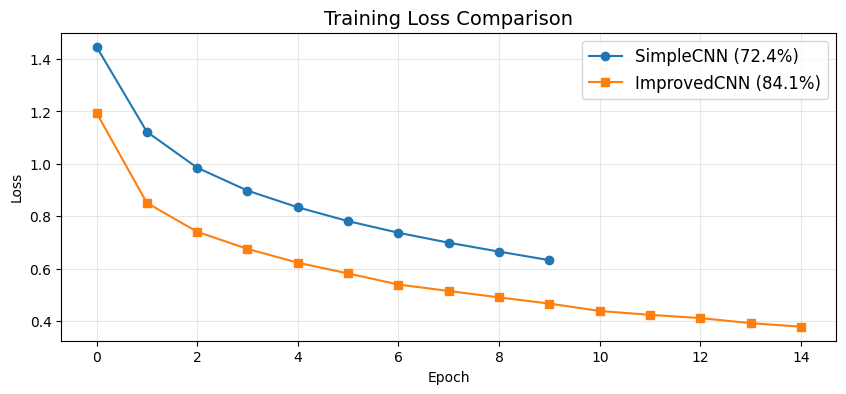
SimpleCNN  final accuracy: 72.40%
ImprovedCNN final accuracy: 84.09%
✅ Check Your Understanding — MCQ Set 6
Q11: What is the PRIMARY benefit of Batch Normalization?
A) It makes the network shallower
B) It stabilizes learning by normalizing layer outputs, allowing higher learning rates
C) It increases the number of parameters dramatically
D) It removes the need for an activation function
Click to reveal solution
Answer: B) It stabilizes learning by normalizing layer outputs, allowing higher learning rates
Q12: How does Dropout help prevent overfitting?
A) It adds more neurons to the network
B) It randomly zeroes out neurons during training, forcing the network to learn robust features
C) It only trains on a subset of the data
D) It increases the learning rate automatically
Click to reveal solution
Answer: B) It randomly zeroes out neurons during training, forcing the network to learn robust features
Q13: Why do deeper CNNs generally learn more complex features?
A) They always train on more data
B) Early layers detect simple patterns (edges); deeper layers combine them into complex patterns (textures, object parts)
C) They use fewer parameters per layer
D) They avoid non-linearities entirely
Click to reveal solution
Answer: B) Early layers detect simple patterns (edges); deeper layers combine them into complex patterns (textures, object parts)
Part 7 — Visualizing What the Network Learns (~10 min)
One of the most powerful things about CNNs: we can actually look inside and see what patterns the network detects. Let’s visualize:
The learned filters (weights of the first conv layer)
The activations (feature maps) when we pass an image through
# ── Visualize first-layer filters (ImprovedCNN) ───────────────────────
kernels = improved_model.conv1.weight.detach().cpu()

fig, axes = plt.subplots(2, 8, figsize=(16, 4))
for i, ax in enumerate(axes.flat):
    if i < kernels.shape[0]:
        k = kernels[i].numpy()  # (3, 3, 3) — RGB filter
        # Normalize each filter for display
        k = (k - k.min()) / (k.max() - k.min() + 1e-8)
        ax.imshow(np.transpose(k, (1, 2, 0)))  # (3, 3, 3) → (3, 3, 3) HWC
        ax.set_title(f'F{i}', fontsize=9)
    ax.axis('off')
plt.suptitle('First Conv Layer Filters (ImprovedCNN) — Each filter detects a different pattern',
             fontsize=13, fontweight='bold')
plt.tight_layout()
plt.show()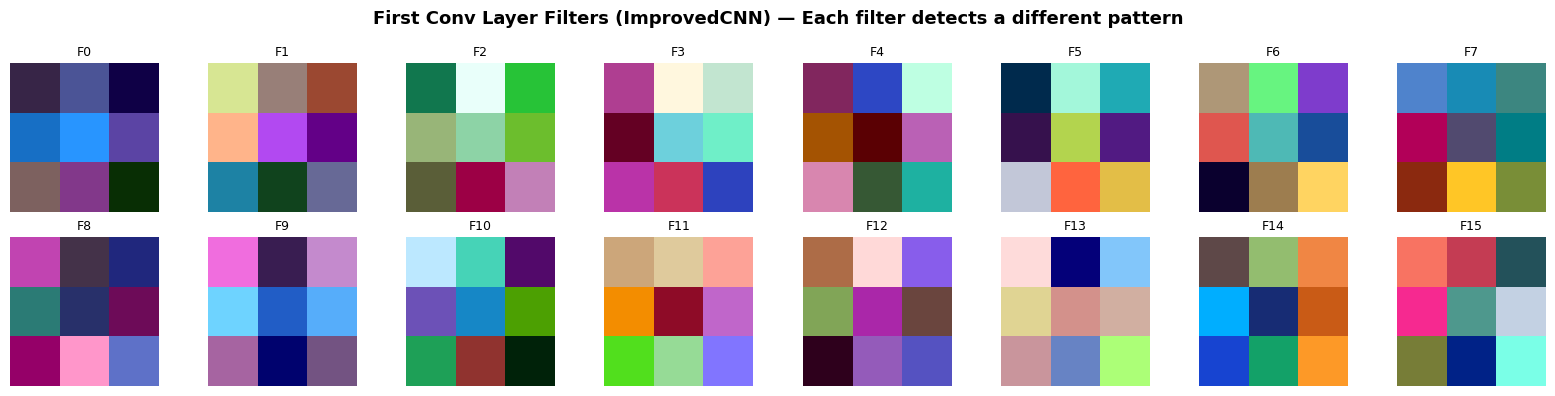
# ── Visualize activations (feature maps) ──────────────────────────────
# Take one test image and pass it through the first conv layer
sample_img, sample_label = test_dataset[0]
sample_batch = sample_img.unsqueeze(0).to(device)  # (1, 3, 32, 32)

# Show the original image
plt.figure(figsize=(3, 3))
img_display = sample_img / 2 + 0.5  # unnormalize
plt.imshow(np.transpose(img_display.numpy(), (1, 2, 0)))
plt.title(f'Input Image: {classes[sample_label]}', fontsize=13)
plt.axis('off')
plt.show()

# Get first-layer activations
improved_model.eval()
with torch.no_grad():
    first_conv_out = F.relu(improved_model.bn1(improved_model.conv1(sample_batch)))

# Show first 16 feature maps
fig, axes = plt.subplots(2, 8, figsize=(16, 4))
for i, ax in enumerate(axes.flat):
    if i < first_conv_out.shape[1]:
        ax.imshow(first_conv_out[0, i].cpu().numpy(), cmap='viridis')
        ax.set_title(f'Map {i}', fontsize=9)
    ax.axis('off')
plt.suptitle('Feature Maps After First Conv Layer — Each map highlights different patterns',
             fontsize=13, fontweight='bold')
plt.tight_layout()
plt.show()

print('🔍 Notice how different feature maps respond to different parts of the image.')
print('   Some might highlight edges, others respond to color regions.')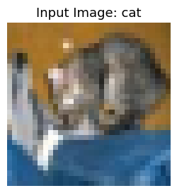
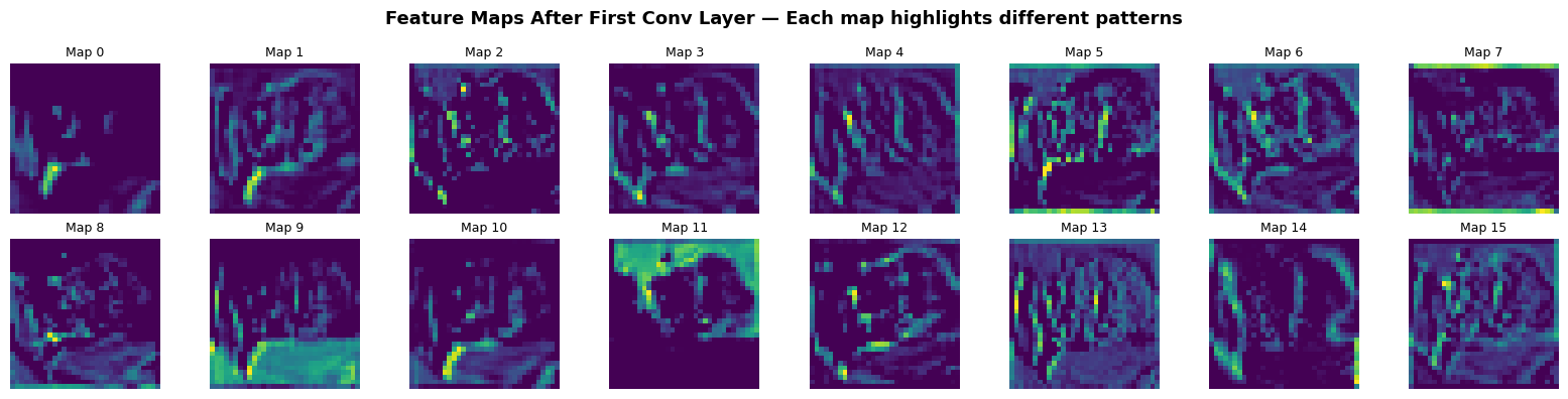
🔍 Notice how different feature maps respond to different parts of the image.
   Some might highlight edges, others respond to color regions.
Per-Class Accuracy
# ── Per-class accuracy ────────────────────────────────────────────────
class_correct = {c: 0 for c in classes}
class_total = {c: 0 for c in classes}

improved_model.eval()
with torch.no_grad():
    for images, labels in test_loader:
        images, labels = images.to(device), labels.to(device)
        preds = improved_model(images).argmax(1)
        for label, pred in zip(labels, preds):
            class_name = classes[label]
            class_total[class_name] += 1
            if label == pred:
                class_correct[class_name] += 1

print('Per-class accuracy (ImprovedCNN):')
print('-' * 35)
for c in classes:
    acc = 100 * class_correct[c] / class_total[c]
    bar = '█' * int(acc / 5) + '░' * (20 - int(acc / 5))
    print(f'{c:12s}  {bar}  {acc:.1f}%')
Per-class accuracy (ImprovedCNN):
-----------------------------------
airplane ████████████████░░░░ 82.7%
automobile ██████████████████░░ 92.3%
bird ██████████████░░░░░░ 74.2%
cat ██████████████░░░░░░ 72.1%
deer ███████████████░░░░░ 76.9%
dog ███████████████░░░░░ 78.1%
frog █████████████████░░░ 88.0%
horse █████████████████░░░ 89.8%
ship ██████████████████░░ 92.3%
truck ██████████████████░░ 94.5%
✅ Check Your Understanding — MCQ Set 7
Q14: Which statement BEST describes a ‘feature map’ in a CNN?
A) The original input image
B) The result of applying one filter across the image, followed by an activation function
C) The final class probabilities
D) The weights of a fully connected layer
Click to reveal solution
Answer: B) The result of applying one filter across the image, followed by an activation function
Q15: What is the key difference between Max Pooling and Average Pooling?
A) Max pooling selects the largest value in each window; average pooling computes the mean
B) Max pooling increases dimensionality; average pooling reduces it
C) They are identical in effect
D) Max pooling only works with grayscale images
Click to reveal solution
Answer: A) Max pooling selects the largest value in each window; average pooling computes the mean
Part 8 — Summary & Key Takeaways
What We Learned Today
| Concept | Key Idea |
|---|---|
| Why CNNs? | MLPs waste parameters on images and ignore spatial structure. CNNs use local connectivity + weight sharing. |
| Convolution | A small filter slides across the image, detecting local patterns. The output is a feature map. |
| ReLU | Adds non-linearity so the network can learn complex patterns. |
| Pooling | Reduces spatial size, makes the network robust to small shifts. Max pooling is most common. |
| Feature Hierarchy | Early layers → edges & textures. Deeper layers → complex shapes & object parts. |
| BatchNorm | Stabilizes training by normalizing layer outputs. |
| Dropout | Prevents overfitting by randomly disabling neurons during training. |
The CNN Recipe
Image → [Conv → BN → ReLU → Pool → Dropout] × N → Flatten → [FC → ReLU → Dropout] × M → Output🎯 Exercises (Try These!)
Easy: Replace
MaxPool2dwithAvgPool2dinSimpleCNNand compare the final accuracy.Medium: Add a third convolutional block to
ImprovedCNN(e.g., 64→128 filters). How does accuracy change?Medium: Try different Dropout rates (0.1 vs 0.5). What happens to training loss vs test accuracy?
Challenge: Try training the
ImprovedCNNwithout BatchNorm. How does training stability change?
✅ Final Self-Assessment
Final Q: A student says ‘CNNs are better than MLPs for images because they have more parameters.’ Is this correct?
A) Yes — more parameters always means better performance
B) No — CNNs actually use FEWER parameters thanks to weight sharing, and they exploit spatial structure
C) Yes — CNNs always have more layers, so more parameters
D) No — MLPs and CNNs have exactly the same number of parameters
Click to reveal solution
Answer: B) No — CNNs actually use FEWER parameters thanks to weight sharing, and they exploit spatial structure