Learning Objectives:
Understand how to prepare and work with time-series data
Build neural networks for sequential prediction
Apply knowledge to a new image dataset (Fashion MNIST)
Compare model architectures for different tasks
Part 1: Introduction to Time-Series Data
What is Time-Series Data?
Time-series data is a sequence of observations recorded at successive time intervals. Examples include:
Stock prices over days/months
Temperature readings over hours
Sales data over quarters
Sensor readings from IoT devices
Key Characteristics:
Temporal Ordering: The order of data points matters
Autocorrelation: Past values influence future values
Trends: Long-term increases or decreases
Seasonality: Repeating patterns at regular intervals
The Prediction Task: Given a sequence of past observations, predict the next value(s).
Part 2: Creating a Synthetic Time-Series Dataset
We’ll create a synthetic dataset that simulates daily temperature with:
A trend (gradual increase)
Seasonality (yearly cycle)
Random noise (natural variation)
import torch
import torch.nn as nn
import torch.optim as optim
from torch.utils.data import Dataset, DataLoader, TensorDataset
import numpy as np
import matplotlib.pyplot as plt
from sklearn.preprocessing import MinMaxScaler

# Set random seeds for reproducibility
torch.manual_seed(42)
np.random.seed(42)
if torch.backends.mps.is_available():
device = torch.device("mps")
print("Using MPS device")
else:
device = torch.device("cpu")
print("MPS not available, using CPU")Using MPS device
# Generate synthetic temperature data
def generate_temperature_data(n_days=1000):
    """
    Generate synthetic daily temperature data with trend, seasonality, and noise
    """
    time = np.arange(n_days)

    # Trend: gradual warming over time
    trend = 0.01 * time

    # Seasonality: yearly cycle (365 days)
    seasonality = 10 * np.sin(2 * np.pi * time / 365)

    # Random noise
    noise = np.random.normal(0, 2, n_days)

    # Base temperature around 20°C
    temperature = 20 + trend + seasonality + noise

    return temperature

# Generate data
temperatures = generate_temperature_data(1000)

# Visualize
plt.figure(figsize=(15, 4))
plt.plot(temperatures[:365], label='First Year')
plt.xlabel('Day')
plt.ylabel('Temperature (°C)')
plt.title('Synthetic Temperature Data')
plt.legend()
plt.grid(True, alpha=0.3)
plt.show()

print(f"Generated {len(temperatures)} days of temperature data")
print(f"Temperature range: {temperatures.min():.2f}°C to {temperatures.max():.2f}°C")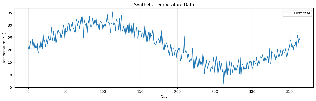
Generated 1000 days of temperature data
Temperature range: 6.34°C to 42.82°C
Part 3: Creating Sequences (Windowing)
The Windowing Approach:
To train a neural network on time-series data, we need to create input-output pairs:
Input: A sequence of past observations (e.g., temperatures from the last 7 days)
Output: The next value to predict (e.g., temperature on day 8)
Example:
Original data: [10, 12, 11, 13, 15, 14, 16, 18, 17, 19, ...]

With window_size = 3:
Input: [10, 12, 11] → Output: 13
Input: [12, 11, 13] → Output: 15
Input: [11, 13, 15] → Output: 14
...
Source
import matplotlib.pyplot as plt
import matplotlib.patches as patches
import numpy as np

# Create a simple time series for demonstration
demo_data = [10, 12, 11, 13, 15, 14, 16, 18, 17, 19, 21, 20]
window_size = 3

# Create figure with two subplots
fig, (ax1, ax2) = plt.subplots(2, 1, figsize=(14, 10))

# ========== Plot 1: Visualizing the sliding window ==========
ax1.plot(range(len(demo_data)), demo_data, 'o-', linewidth=2, markersize=8, color='steelblue', label='Time Series Data')
ax1.set_xlabel('Time Step', fontsize=12)
ax1.set_ylabel('Value', fontsize=12)
ax1.set_title('Sliding Window Approach for Time-Series Prediction', fontsize=14, fontweight='bold')
ax1.grid(True, alpha=0.3)
ax1.set_xlim(-0.5, len(demo_data)-0.5)

# Show first 3 windows with different colors
colors = ['#FF6B6B', '#4ECDC4', '#95E1D3']
window_labels = ['Window 1', 'Window 2', 'Window 3']

for w_idx in range(3):
    # Highlight input window
    for i in range(window_size):
        idx = w_idx + i
        rect = patches.Rectangle((idx-0.3, demo_data[idx]-0.5), 0.6, 1,
                                linewidth=2, edgecolor=colors[w_idx],
                                facecolor=colors[w_idx], alpha=0.3)
        ax1.add_patch(rect)

    # Highlight output (next value)
    output_idx = w_idx + window_size
    rect = patches.Rectangle((output_idx-0.3, demo_data[output_idx]-0.5), 0.6, 1,
                            linewidth=3, edgecolor=colors[w_idx],
                            facecolor='none', linestyle='--')
    ax1.add_patch(rect)

    # Add arrows and labels
    mid_x = w_idx + window_size/2 - 0.5
    ax1.annotate('', xy=(output_idx, demo_data[output_idx]),
                xytext=(mid_x, demo_data[output_idx]),
                arrowprops=dict(arrowstyle='->', color=colors[w_idx], lw=2))

    # Label the window
    ax1.text(mid_x, max(demo_data) + 1.5 - w_idx*0.8, window_labels[w_idx],
            fontsize=11, fontweight='bold', color=colors[w_idx],
            ha='center', bbox=dict(boxstyle='round,pad=0.3', facecolor='white', alpha=0.8))

# Add legend elements
ax1.plot([], [], 's', markersize=15, color='steelblue', alpha=0.3, label='Input Window')
ax1.plot([], [], 's', markersize=15, markerfacecolor='none', markeredgecolor='black',
         markeredgewidth=2, linestyle='--', label='Target (Output)')
ax1.legend(loc='upper left', fontsize=11)

# ========== Plot 2: Show all input-output pairs in a table format ==========
ax2.axis('off')
ax2.set_xlim(0, 10)
ax2.set_ylim(0, 10)
ax2.set_title('All Input-Output Pairs Created from Windowing', fontsize=14, fontweight='bold', pad=20)

# Create table-like visualization
y_start = 8.5
y_step = 0.9

# Header
ax2.text(2, y_start, 'Input Sequence', fontsize=12, fontweight='bold', ha='center',
         bbox=dict(boxstyle='round,pad=0.5', facecolor='lightblue', alpha=0.8))
ax2.text(6.5, y_start, '→', fontsize=16, ha='center', fontweight='bold')
ax2.text(8.5, y_start, 'Target', fontsize=12, fontweight='bold', ha='center',
         bbox=dict(boxstyle='round,pad=0.5', facecolor='lightcoral', alpha=0.8))

# Generate and display all sequences
y_pos = y_start - y_step
for i in range(len(demo_data) - window_size):
    input_seq = demo_data[i:i+window_size]
    output_val = demo_data[i+window_size]

    # Input sequence
    input_str = f"[{', '.join(map(str, input_seq))}]"
    ax2.text(2, y_pos, input_str, fontsize=11, ha='center',
            bbox=dict(boxstyle='round,pad=0.3', facecolor='white', edgecolor='steelblue', linewidth=1.5))

    # Arrow
    ax2.text(6.5, y_pos, '→', fontsize=14, ha='center', color='gray')

    # Output value
    ax2.text(8.5, y_pos, str(output_val), fontsize=11, ha='center',
            bbox=dict(boxstyle='round,pad=0.3', facecolor='white', edgecolor='coral', linewidth=1.5))

    y_pos -= y_step

    if y_pos < 0.5:  # Stop if we run out of space
        break

# Add summary text
summary_text = f"Window Size = {window_size}\nTotal Sequences Created: {len(demo_data) - window_size}"
ax2.text(5, 0.2, summary_text, fontsize=11, ha='center',
        bbox=dict(boxstyle='round,pad=0.5', facecolor='lightyellow', alpha=0.8))

plt.tight_layout()
plt.show()

# Print explanation
print("=" * 70)
print("WINDOWING CONCEPT EXPLAINED")
print("=" * 70)
print(f"Original time series: {demo_data}")
print(f"\nWith window_size = {window_size}:")
print(f"  - Each input contains {window_size} consecutive values")
print(f"  - Each output is the next value after the window")
print(f"  - Total training examples created: {len(demo_data) - window_size}")
print("\nThis sliding window approach allows us to:")
print("  1. Convert time-series into supervised learning format")
print("  2. Use past observations to predict future values")
print("  3. Create multiple training examples from one sequence")
print("=" * 70)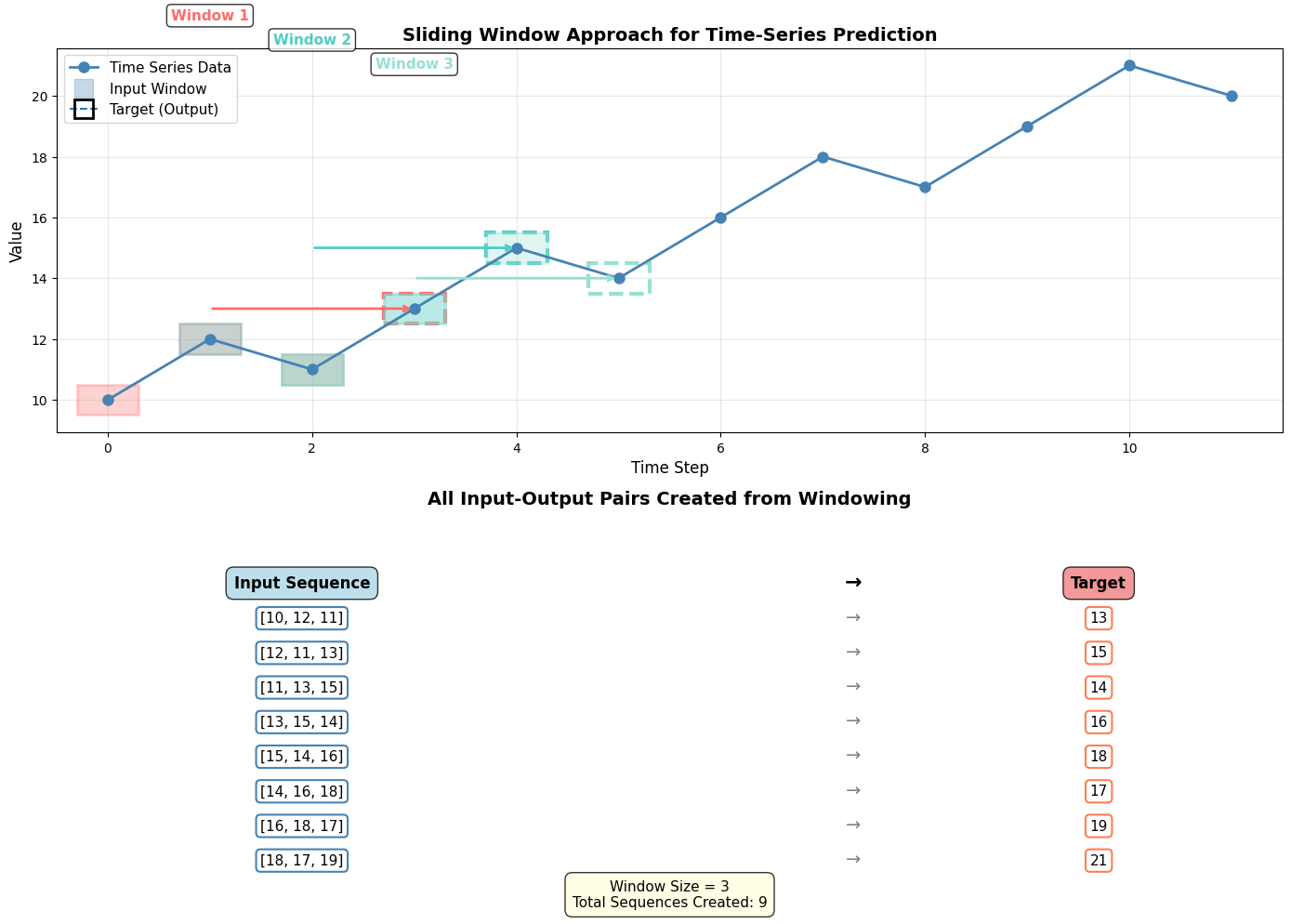
======================================================================
WINDOWING CONCEPT EXPLAINED
======================================================================
Original time series: [10, 12, 11, 13, 15, 14, 16, 18, 17, 19, 21, 20]

With window_size = 3:
  - Each input contains 3 consecutive values
  - Each output is the next value after the window
  - Total training examples created: 9

This sliding window approach allows us to:
  1. Convert time-series into supervised learning format
  2. Use past observations to predict future values
  3. Create multiple training examples from one sequence
======================================================================
def create_sequences(data, window_size):
    """
    Create input-output pairs for time-series prediction

    Args:
        data: 1D array of time-series values
        window_size: Number of past observations to use for prediction

    Returns:
        X: Input sequences (n_samples, window_size)
        y: Target values (n_samples,)
    """
    X, y = [], []

    for i in range(len(data) - window_size):
        # Input: window_size past observations
        X.append(data[i:i + window_size])
        # Output: next value
        y.append(data[i + window_size])

    return np.array(X), np.array(y)

# Create sequences with window size of 7 days
window_size = 7
X, y = create_sequences(temperatures, window_size)

print(f"Created {len(X)} sequences")
print(f"Input shape: {X.shape}")
print(f"Output shape: {y.shape}")
print(f"\nExample:")
print(f"Input (7 days): {X[0]}")
print(f"Output (next day): {y[0]:.2f}")
Created 993 sequences
Input shape: (993, 7)
Output shape: (993,)
Example:
Input (7 days): [20.99342831 19.90560496 21.65959319 23.59225639 20.25971752 20.44137407
24.24944261]
Output (next day): 22.81
Part 4: Normalize and Split Data
Why Normalize?
Neural networks train better with normalized inputs (values between 0 and 1, or -1 and 1)
Prevents features with larger scales from dominating
Helps with gradient flow during backpropagation
Important: Scale on training data only, then apply to test data to prevent data leakage!
# Split into train and test (80-20)
train_size = int(0.8 * len(X))
X_train, X_test = X[:train_size], X[train_size:]
y_train, y_test = y[:train_size], y[train_size:]

# Normalize using MinMaxScaler
scaler_X = MinMaxScaler()
scaler_y = MinMaxScaler()

# Fit on training data only!
X_train_scaled = scaler_X.fit_transform(X_train)
X_test_scaled = scaler_X.transform(X_test)

y_train_scaled = scaler_y.fit_transform(y_train.reshape(-1, 1)).flatten()
y_test_scaled = scaler_y.transform(y_test.reshape(-1, 1)).flatten()

# Convert to PyTorch tensors
X_train_tensor = torch.FloatTensor(X_train_scaled)
y_train_tensor = torch.FloatTensor(y_train_scaled)
X_test_tensor = torch.FloatTensor(X_test_scaled)
y_test_tensor = torch.FloatTensor(y_test_scaled)

print(f"Training samples: {len(X_train_tensor)}")
print(f"Test samples: {len(X_test_tensor)}")
print(f"\nScaled value range: [{X_train_scaled.min():.3f}, {X_train_scaled.max():.3f}]")
Training samples: 794
Test samples: 199
Scaled value range: [0.000, 1.000]
# Create DataLoaders
train_dataset = TensorDataset(X_train_tensor, y_train_tensor)
test_dataset = TensorDataset(X_test_tensor, y_test_tensor)

train_loader = DataLoader(train_dataset, batch_size=32, shuffle=True)
test_loader = DataLoader(test_dataset, batch_size=32, shuffle=False)

print(f"Created DataLoaders with batch size 32")
print(f"Number of batches in train_loader: {len(train_loader)}")
Created DataLoaders with batch size 32
Number of batches in train_loader: 25
Part 5: Building a Time-Series Prediction Model
We’ll build a simple feedforward neural network for time-series prediction:
Architecture:
Input: 7 past temperature values
Hidden Layer 1: 64 neurons (ReLU)
Hidden Layer 2: 32 neurons (ReLU)
Output: 1 predicted temperature value
Note: For more complex time-series, you’d typically use RNNs or LSTMs, but this simple architecture works well for our data!
class TimeSeriesNet(nn.Module):
    def __init__(self, input_size, hidden_size1=64, hidden_size2=32):
        super(TimeSeriesNet, self).__init__()

        self.network = nn.Sequential(
            nn.Linear(input_size, hidden_size1),
            nn.ReLU(),
            nn.Linear(hidden_size1, hidden_size2),
            nn.ReLU(),
            nn.Linear(hidden_size2, 1)
        )

    def forward(self, x):
        return self.network(x).squeeze()

# Instantiate the model
model = TimeSeriesNet(input_size=window_size)
print(model)

# Count parameters
total_params = sum(p.numel() for p in model.parameters())
print(f"\nTotal parameters: {total_params:,}")
TimeSeriesNet(
(network): Sequential(
(0): Linear(in_features=7, out_features=64, bias=True)
(1): ReLU()
(2): Linear(in_features=64, out_features=32, bias=True)
(3): ReLU()
(4): Linear(in_features=32, out_features=1, bias=True)
)
)
Total parameters: 2,625
Part 6: Training the Model
# Define loss and optimizer
criterion = nn.MSELoss()
optimizer = optim.Adam(model.parameters(), lr=0.001)

# Training loop
num_epochs = 100
train_losses = []
val_losses = []

for epoch in range(num_epochs):
    # Training phase
    model.train()
    train_loss = 0.0

    for inputs, targets in train_loader:
        # Forward pass
        outputs = model(inputs)
        loss = criterion(outputs, targets)

        # Backward pass and optimize
        optimizer.zero_grad()
        loss.backward()
        optimizer.step()

        train_loss += loss.item() * inputs.size(0)

    train_loss = train_loss / len(train_loader.dataset)
    train_losses.append(train_loss)

    # Validation phase
    model.eval()
    val_loss = 0.0

    with torch.no_grad():
        for inputs, targets in test_loader:
            outputs = model(inputs)
            loss = criterion(outputs, targets)
            val_loss += loss.item() * inputs.size(0)

    val_loss = val_loss / len(test_loader.dataset)
    val_losses.append(val_loss)

    if (epoch + 1) % 5 == 0:
        print(f'Epoch [{epoch+1}/{num_epochs}], Train Loss: {train_loss:.6f}, Val Loss: {val_loss:.6f}')

print("\nTraining complete!")
Epoch [5/100], Train Loss: 0.005782, Val Loss: 0.004132
Epoch [10/100], Train Loss: 0.004266, Val Loss: 0.003624
Epoch [15/100], Train Loss: 0.004180, Val Loss: 0.003639
Epoch [20/100], Train Loss: 0.004134, Val Loss: 0.003813
Epoch [25/100], Train Loss: 0.004108, Val Loss: 0.003751
Epoch [30/100], Train Loss: 0.004056, Val Loss: 0.003654
Epoch [35/100], Train Loss: 0.004112, Val Loss: 0.003653
Epoch [40/100], Train Loss: 0.004363, Val Loss: 0.003713
Epoch [45/100], Train Loss: 0.004079, Val Loss: 0.003709
Epoch [50/100], Train Loss: 0.004094, Val Loss: 0.004127
Epoch [55/100], Train Loss: 0.004111, Val Loss: 0.003867
Epoch [60/100], Train Loss: 0.004401, Val Loss: 0.003742
Epoch [65/100], Train Loss: 0.004152, Val Loss: 0.003681
Epoch [70/100], Train Loss: 0.004043, Val Loss: 0.003893
Epoch [75/100], Train Loss: 0.004224, Val Loss: 0.003682
Epoch [80/100], Train Loss: 0.004133, Val Loss: 0.003816
Epoch [85/100], Train Loss: 0.004079, Val Loss: 0.003678
Epoch [90/100], Train Loss: 0.004028, Val Loss: 0.003686
Epoch [95/100], Train Loss: 0.004052, Val Loss: 0.004391
Epoch [100/100], Train Loss: 0.004120, Val Loss: 0.003687
Training complete!
import plotly.express as px
import pandas as pd

# Create a DataFrame with the training history
history_df = pd.DataFrame({
    'Epoch': list(range(1, len(train_losses) + 1)),
    'Training Loss': train_losses,
    'Validation Loss': val_losses
})

# Melt the DataFrame for easier plotting
history_melted = history_df.melt(
    id_vars=['Epoch'],
    value_vars=['Training Loss', 'Validation Loss'],
    var_name='Loss Type',
    value_name='Loss (MSE)'
)

# Create interactive plot
fig = px.line(
    history_melted,
    x='Epoch',
    y='Loss (MSE)',
    color='Loss Type',
    title='Training History - Time-Series Model',
    labels={'Loss (MSE)': 'Loss (MSE)', 'Epoch': 'Epoch'},
    template='plotly_white'
)

fig.update_traces(line=dict(width=2))
fig.update_layout(
    hovermode='x unified',
    legend=dict(yanchor="top", y=0.99, xanchor="right", x=0.99)
)

fig.show()Part 7: Evaluating Predictions
# Make predictions on test set
model.eval()
with torch.no_grad():
predictions_scaled = model(X_test_tensor).numpy()
# Inverse transform to get actual temperature values
predictions = scaler_y.inverse_transform(predictions_scaled.reshape(-1, 1)).flatten()
actuals = scaler_y.inverse_transform(y_test_scaled.reshape(-1, 1)).flatten()
# Calculate metrics
from sklearn.metrics import mean_squared_error, mean_absolute_error, r2_score
mse = mean_squared_error(actuals, predictions)
rmse = np.sqrt(mse)
mae = mean_absolute_error(actuals, predictions)
r2 = r2_score(actuals, predictions)
print("=" * 50)
print("Model Performance on Test Set")
print("=" * 50)
print(f"Mean Squared Error (MSE): {mse:.4f}")
print(f"Root Mean Squared Error (RMSE): {rmse:.4f}°C")
print(f"Mean Absolute Error (MAE): {mae:.4f}°C")
print(f"R² Score: {r2:.4f}")
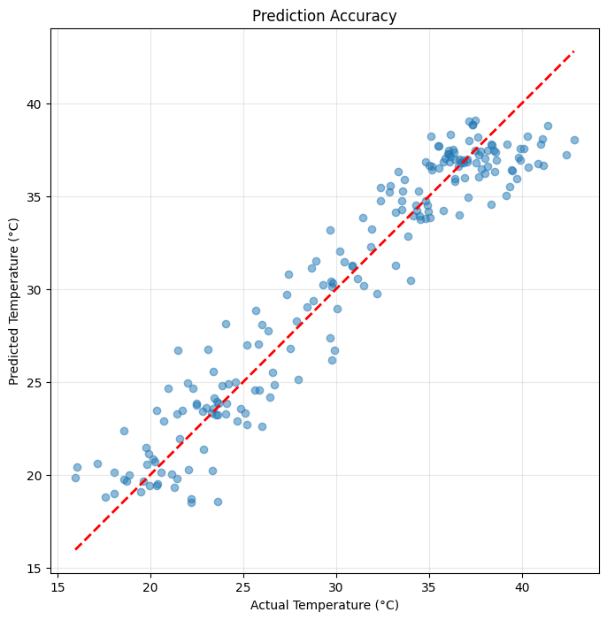
print("=" * 50)==================================================
Model Performance on Test Set
==================================================
Mean Squared Error (MSE): 4.2384
Root Mean Squared Error (RMSE): 2.0587°C
Mean Absolute Error (MAE): 1.6631°C
R² Score: 0.9159
==================================================
# Visualize predictions vs actual values
plt.figure(figsize=(15, 5))

# Plot first 100 predictions
n_plot = 100
plt.plot(actuals[:n_plot], label='Actual', marker='o', markersize=3, alpha=0.7)
plt.plot(predictions[:n_plot], label='Predicted', marker='x', markersize=3, alpha=0.7)
plt.xlabel('Time Step')
plt.ylabel('Temperature (°C)')
plt.title('Temperature Prediction: Actual vs Predicted')
plt.legend()
plt.grid(True, alpha=0.3)
plt.show()

# Scatter plot
plt.figure(figsize=(8, 8))
plt.scatter(actuals, predictions, alpha=0.5)
plt.plot([actuals.min(), actuals.max()], [actuals.min(), actuals.max()], 'r--', lw=2)
plt.xlabel('Actual Temperature (°C)')
plt.ylabel('Predicted Temperature (°C)')
plt.title('Prediction Accuracy')
plt.grid(True, alpha=0.3)
plt.axis('equal')
plt.show()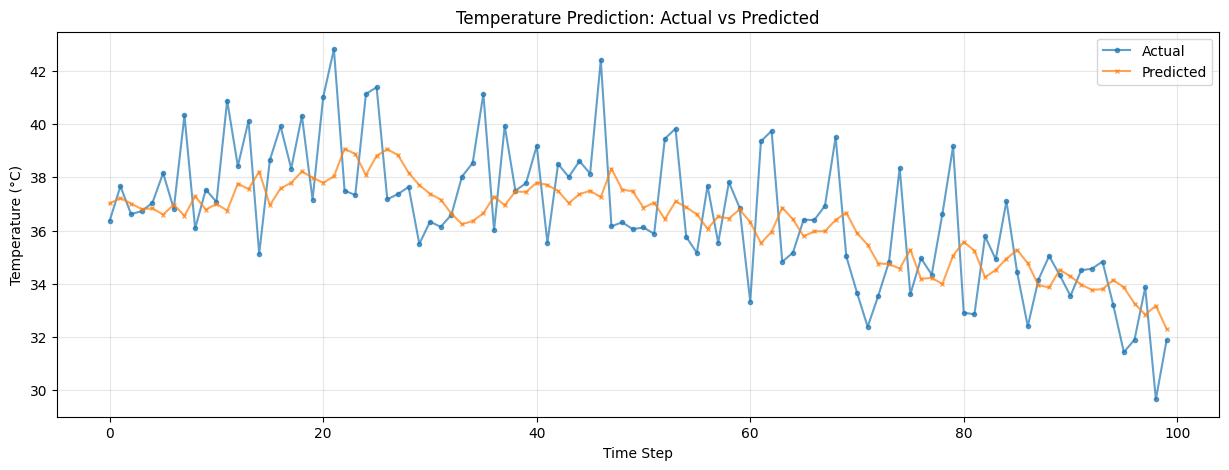
Part 8: Fashion MNIST Classification
Now let’s apply our knowledge to a new image dataset: Fashion MNIST
What is Fashion MNIST?
A dataset of 70,000 grayscale images (28×28 pixels)
10 classes of clothing items instead of digits
Same format as MNIST, but more challenging
Classes: 0. T-shirt/top
Trouser
Pullover
Dress
Coat
Sandal
Shirt
Sneaker
Bag
Ankle boot
Part 9: Loading Fashion MNIST
from torchvision import datasets, transforms

# Define transformations
transform = transforms.Compose([
    transforms.ToTensor(),
    transforms.Normalize((0.5,), (0.5,))
])

# Load Fashion MNIST
fashion_train = datasets.FashionMNIST(
    root='./data',
    train=True,
    download=True,
    transform=transform
)

fashion_test = datasets.FashionMNIST(
    root='./data',
    train=False,
    download=True,
    transform=transform
)

# Create data loaders
fashion_train_loader = DataLoader(fashion_train, batch_size=256, shuffle=True, num_workers=4, persistent_workers=True)
fashion_test_loader = DataLoader(fashion_test, batch_size=256, shuffle=False, num_workers=4, persistent_workers=True)

print(f"Training samples: {len(fashion_train)}")
print(f"Test samples: {len(fashion_test)}")

# Class names
class_names = ['T-shirt/top', 'Trouser', 'Pullover', 'Dress', 'Coat',
               'Sandal', 'Shirt', 'Sneaker', 'Bag', 'Ankle boot']
Training samples: 60000
Test samples: 10000
# Visualize some samples
fig, axes = plt.subplots(2, 5, figsize=(12, 5))
axes = axes.ravel()

for i in range(10):
    img, label = fashion_train[i]
    axes[i].imshow(img.squeeze(), cmap='gray')
    axes[i].set_title(f'{class_names[label]}')
    axes[i].axis('off')

plt.tight_layout()
plt.show()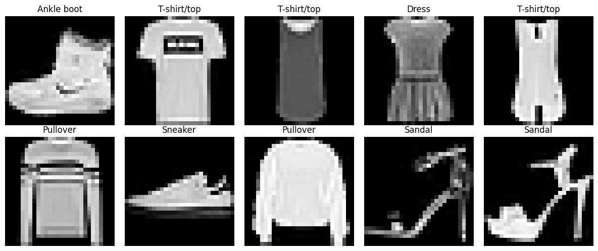
Part 10: Building a Fashion Classifier
We’ll build two models and compare their performance:
Simple MLP (similar to what we used for MNIST)
Deeper MLP with more hidden layers
class SimpleFashionNet(nn.Module):
    """Simple 2-layer MLP"""
    def __init__(self):
        super(SimpleFashionNet, self).__init__()
        self.network = nn.Sequential(
            nn.Flatten(),
            nn.Linear(28*28, 128),
            nn.ReLU(),
            nn.Linear(128, 10)
        )

    def forward(self, x):
        return self.network(x)

class DeepFashionNet(nn.Module):
    """Deeper MLP with dropout"""
    def __init__(self):
        super(DeepFashionNet, self).__init__()
        self.network = nn.Sequential(
            nn.Flatten(),
            nn.Linear(28*28, 256),
            nn.ReLU(),
            nn.Dropout(0.2),
            nn.Linear(256, 128),
            nn.ReLU(),
            nn.Dropout(0.2),
            nn.Linear(128, 64),
            nn.ReLU(),
            nn.Linear(64, 10)
        )

    def forward(self, x):
        return self.network(x)

# Create models
simple_model = SimpleFashionNet().to(device)
deep_model = DeepFashionNet().to(device)

print("Simple Model:")
print(simple_model)
print(f"Parameters: {sum(p.numel() for p in simple_model.parameters()):,}\n")

print("Deep Model:")
print(deep_model)
print(f"Parameters: {sum(p.numel() for p in deep_model.parameters()):,}")
Simple Model:
SimpleFashionNet(
(network): Sequential(
(0): Flatten(start_dim=1, end_dim=-1)
(1): Linear(in_features=784, out_features=128, bias=True)
(2): ReLU()
(3): Linear(in_features=128, out_features=10, bias=True)
)
)
Parameters: 101,770
Deep Model:
DeepFashionNet(
(network): Sequential(
(0): Flatten(start_dim=1, end_dim=-1)
(1): Linear(in_features=784, out_features=256, bias=True)
(2): ReLU()
(3): Dropout(p=0.2, inplace=False)
(4): Linear(in_features=256, out_features=128, bias=True)
(5): ReLU()
(6): Dropout(p=0.2, inplace=False)
(7): Linear(in_features=128, out_features=64, bias=True)
(8): ReLU()
(9): Linear(in_features=64, out_features=10, bias=True)
)
)
Parameters: 242,762
Part 11: Training Both Models
Let’s create a reusable training function:
def train_model(model, train_loader, test_loader, num_epochs=10, lr=0.001):
    """
    Train a model and return training history
    """
    criterion = nn.CrossEntropyLoss()
    optimizer = optim.Adam(model.parameters(), lr=lr)

    train_losses = []
    val_losses = []
    val_accuracies = []

    for epoch in range(num_epochs):
        # Training phase
        model.train()
        train_loss = 0.0

        for images, labels in train_loader:
            images, labels = images.to(device), labels.to(device)
            outputs = model(images)
            loss = criterion(outputs, labels)

            optimizer.zero_grad()
            loss.backward()
            optimizer.step()

            train_loss += loss.item() * images.size(0)

        train_loss = train_loss / len(train_loader.dataset)
        train_losses.append(train_loss)

        # Validation phase
        model.eval()
        val_loss = 0.0
        correct = 0
        total = 0

        with torch.no_grad():
            for images, labels in test_loader:
                images, labels = images.to(device), labels.to(device)
                outputs = model(images)
                loss = criterion(outputs, labels)
                val_loss += loss.item() * images.size(0)

                _, predicted = torch.max(outputs, 1)
                total += labels.size(0)
                correct += (predicted == labels).sum().item()

        val_loss = val_loss / len(test_loader.dataset)
        val_accuracy = 100 * correct / total

        val_losses.append(val_loss)
        val_accuracies.append(val_accuracy)

        print(f'Epoch [{epoch+1}/{num_epochs}], '
              f'Train Loss: {train_loss:.4f}, '
              f'Val Loss: {val_loss:.4f}, '
              f'Val Acc: {val_accuracy:.2f}%')

    return train_losses, val_losses, val_accuracies
print("Training Simple Model...")
print("=" * 70)
simple_train_losses, simple_val_losses, simple_val_accs = train_model(
simple_model, fashion_train_loader, fashion_test_loader, num_epochs=15
)
print("\n" + "=" * 70)Training Simple Model...
======================================================================
Epoch [1/15], Train Loss: 0.5782, Val Loss: 0.4691, Val Acc: 83.00%
Epoch [2/15], Train Loss: 0.4134, Val Loss: 0.4207, Val Acc: 84.76%
Epoch [3/15], Train Loss: 0.3688, Val Loss: 0.4090, Val Acc: 85.41%
Epoch [4/15], Train Loss: 0.3473, Val Loss: 0.4026, Val Acc: 85.56%
Epoch [5/15], Train Loss: 0.3267, Val Loss: 0.3902, Val Acc: 85.97%
Epoch [6/15], Train Loss: 0.3092, Val Loss: 0.3617, Val Acc: 87.08%
Epoch [7/15], Train Loss: 0.2954, Val Loss: 0.3480, Val Acc: 87.72%
Epoch [8/15], Train Loss: 0.2864, Val Loss: 0.3629, Val Acc: 86.83%
Epoch [9/15], Train Loss: 0.2746, Val Loss: 0.3534, Val Acc: 87.35%
Epoch [10/15], Train Loss: 0.2673, Val Loss: 0.3333, Val Acc: 88.34%
Epoch [11/15], Train Loss: 0.2548, Val Loss: 0.3294, Val Acc: 88.32%
Epoch [12/15], Train Loss: 0.2464, Val Loss: 0.3498, Val Acc: 88.05%
Epoch [13/15], Train Loss: 0.2416, Val Loss: 0.3313, Val Acc: 88.06%
Epoch [14/15], Train Loss: 0.2362, Val Loss: 0.3309, Val Acc: 88.43%
Epoch [15/15], Train Loss: 0.2267, Val Loss: 0.3334, Val Acc: 88.37%
======================================================================
print("\nTraining Deep Model...")
print("=" * 70)
deep_train_losses, deep_val_losses, deep_val_accs = train_model(
    deep_model, fashion_train_loader, fashion_test_loader, num_epochs=15
)
print("\n" + "=" * 70)
Training Deep Model...
======================================================================
Epoch [1/15], Train Loss: 0.6717, Val Loss: 0.4649, Val Acc: 82.92%
Epoch [2/15], Train Loss: 0.4324, Val Loss: 0.4110, Val Acc: 85.04%
Epoch [3/15], Train Loss: 0.3869, Val Loss: 0.3933, Val Acc: 85.86%
Epoch [4/15], Train Loss: 0.3599, Val Loss: 0.3781, Val Acc: 86.48%
Epoch [5/15], Train Loss: 0.3389, Val Loss: 0.3733, Val Acc: 86.44%
Epoch [6/15], Train Loss: 0.3262, Val Loss: 0.3593, Val Acc: 87.16%
Epoch [7/15], Train Loss: 0.3166, Val Loss: 0.3605, Val Acc: 86.91%
Epoch [8/15], Train Loss: 0.3012, Val Loss: 0.3428, Val Acc: 87.51%
Epoch [9/15], Train Loss: 0.2932, Val Loss: 0.3414, Val Acc: 87.86%
Epoch [10/15], Train Loss: 0.2843, Val Loss: 0.3523, Val Acc: 87.29%
Epoch [11/15], Train Loss: 0.2793, Val Loss: 0.3239, Val Acc: 88.33%
Epoch [12/15], Train Loss: 0.2725, Val Loss: 0.3410, Val Acc: 88.16%
Epoch [13/15], Train Loss: 0.2639, Val Loss: 0.3297, Val Acc: 88.35%
Epoch [14/15], Train Loss: 0.2604, Val Loss: 0.3293, Val Acc: 88.31%
Epoch [15/15], Train Loss: 0.2533, Val Loss: 0.3218, Val Acc: 88.65%

======================================================================
Part 12: Comparing Model Performance
import plotly.graph_objects as go
from plotly.subplots import make_subplots
import pandas as pd

# Create a DataFrame with all the data
comparison_df = pd.DataFrame({
    'Epoch': list(range(1, len(simple_train_losses) + 1)),
    'Simple_Train': simple_train_losses,
    'Simple_Val': simple_val_losses,
    'Simple_Acc': simple_val_accs,
    'Deep_Train': deep_train_losses,
    'Deep_Val': deep_val_losses,
    'Deep_Acc': deep_val_accs
})

# Create subplots
fig = make_subplots(
    rows=1, cols=3,
    subplot_titles=('Training Loss Comparison',
                    'Validation Loss Comparison',
                    'Validation Accuracy Comparison'),
    horizontal_spacing=0.1
)

# Plot 1: Training Loss
fig.add_trace(
    go.Scatter(x=comparison_df['Epoch'], y=comparison_df['Simple_Train'],
               mode='lines+markers', name='Simple Model',
               marker=dict(size=4), line=dict(width=2),
               legendgroup='simple'),
    row=1, col=1
)
fig.add_trace(
    go.Scatter(x=comparison_df['Epoch'], y=comparison_df['Deep_Train'],
               mode='lines+markers', name='Deep Model',
               marker=dict(size=4, symbol='square'), line=dict(width=2),
               legendgroup='deep'),
    row=1, col=1
)

# Plot 2: Validation Loss
fig.add_trace(
    go.Scatter(x=comparison_df['Epoch'], y=comparison_df['Simple_Val'],
               mode='lines+markers', name='Simple Model',
               marker=dict(size=4), line=dict(width=2),
               legendgroup='simple', showlegend=False),
    row=1, col=2
)
fig.add_trace(
    go.Scatter(x=comparison_df['Epoch'], y=comparison_df['Deep_Val'],
               mode='lines+markers', name='Deep Model',
               marker=dict(size=4, symbol='square'), line=dict(width=2),
               legendgroup='deep', showlegend=False),
    row=1, col=2
)

# Plot 3: Validation Accuracy
fig.add_trace(
    go.Scatter(x=comparison_df['Epoch'], y=comparison_df['Simple_Acc'],
               mode='lines+markers', name='Simple Model',
               marker=dict(size=4), line=dict(width=2),
               legendgroup='simple', showlegend=False),
    row=1, col=3
)
fig.add_trace(
    go.Scatter(x=comparison_df['Epoch'], y=comparison_df['Deep_Acc'],
               mode='lines+markers', name='Deep Model',
               marker=dict(size=4, symbol='square'), line=dict(width=2),
               legendgroup='deep', showlegend=False),
    row=1, col=3
)

# Update axes labels
fig.update_xaxes(title_text="Epoch", row=1, col=1)
fig.update_xaxes(title_text="Epoch", row=1, col=2)
fig.update_xaxes(title_text="Epoch", row=1, col=3)

fig.update_yaxes(title_text="Loss", row=1, col=1)
fig.update_yaxes(title_text="Loss", row=1, col=2)
fig.update_yaxes(title_text="Accuracy (%)", row=1, col=3)

# Update layout
fig.update_layout(
    height=400,
    width=1400,
    template='plotly_white',
    hovermode='x unified',
    legend=dict(
        yanchor="top",
        y=0.99,
        xanchor="left",
        x=0.01,
        orientation="v"
    )
)

fig.show()

# Print final results
print("\n" + "=" * 70)
print("FINAL RESULTS")
print("=" * 70)
print(f"Simple Model - Final Val Accuracy: {simple_val_accs[-1]:.2f}%")
print(f"Deep Model   - Final Val Accuracy: {deep_val_accs[-1]:.2f}%")
print(f"\nImprovement: {deep_val_accs[-1] - simple_val_accs[-1]:.2f}%")
print("=" * 70)
======================================================================
FINAL RESULTS
======================================================================
Simple Model - Final Val Accuracy: 88.37%
Deep Model   - Final Val Accuracy: 88.65%

Improvement: 0.28%
======================================================================
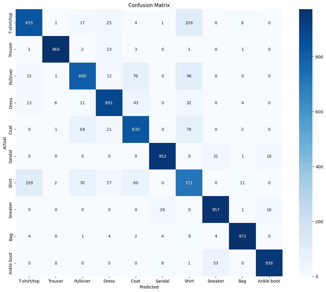
Part 13: Detailed Analysis - Confusion Matrix
from sklearn.metrics import confusion_matrix
import seaborn as sns

def plot_confusion_matrix(model, test_loader, class_names):
    """
    Create and plot confusion matrix
    """
    model.eval()
    all_preds = []
    all_labels = []

    with torch.no_grad():
        for images, labels in test_loader:
            images, labels = images.to(device), labels.to(device)
            outputs = model(images)
            _, predicted = torch.max(outputs, 1)
            all_preds.extend(predicted.cpu().numpy())
            all_labels.extend(labels.cpu().numpy())

    # Create confusion matrix
    cm = confusion_matrix(all_labels, all_preds)

    # Plot
    plt.figure(figsize=(12, 10))
    sns.heatmap(cm, annot=True, fmt='d', cmap='Blues',
                xticklabels=class_names,
                yticklabels=class_names)
    plt.xlabel('Predicted')
    plt.ylabel('Actual')
    plt.title('Confusion Matrix')
    plt.tight_layout()
    plt.show()

    return cm

print("Confusion Matrix for Deep Model:")
cm = plot_confusion_matrix(deep_model, fashion_test_loader, class_names)
Confusion Matrix for Deep Model:
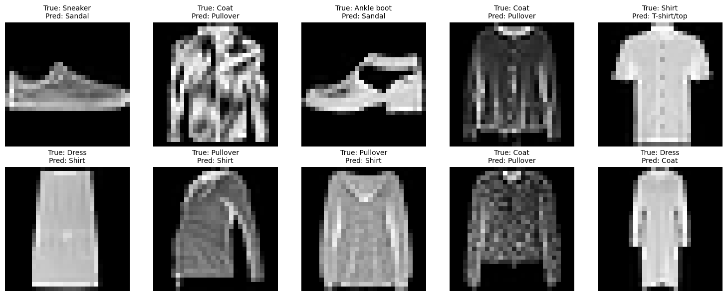
Part 14: Error Analysis - What Does the Model Get Wrong?
def show_misclassifications(model, test_loader, class_names, num_examples=10):
    """
    Display examples of misclassified images
    """
    model.eval()
    misclassified = []

    with torch.no_grad():
        for images, labels in test_loader:
            images, labels = images.to(device), labels.to(device)
            outputs = model(images)
            _, predicted = torch.max(outputs, 1)

            # Find misclassified examples
            mask = predicted != labels
            for i, is_wrong in enumerate(mask):
                if is_wrong:
                    misclassified.append({
                        'image': images[i].cpu(),  # Move to CPU here
                        'true': labels[i].item(),
                        'pred': predicted[i].item()
                    })

            if len(misclassified) >= num_examples:
                break

    # Plot
    fig, axes = plt.subplots(2, 5, figsize=(15, 6))
    axes = axes.ravel()

    for i in range(min(num_examples, len(misclassified))):
        img = misclassified[i]['image'].squeeze()
        true_label = class_names[misclassified[i]['true']]
        pred_label = class_names[misclassified[i]['pred']]

        axes[i].imshow(img, cmap='gray')
        axes[i].set_title(f'True: {true_label}\nPred: {pred_label}', fontsize=10)
        axes[i].axis('off')

    plt.tight_layout()
    plt.show()

print("Examples of Misclassified Images:")
show_misclassifications(deep_model, fashion_test_loader, class_names)
Examples of Misclassified Images:
Summary and Key Takeaways
Time-Series Prediction
Data Preparation: Creating sequences with windowing is crucial
Normalization: Always normalize time-series data
Train-Test Split: Respect temporal ordering (no random shuffle)
Metrics: RMSE and MAE are more interpretable than MSE for regression
Fashion MNIST Classification
Transfer Knowledge: Skills from MNIST transfer to Fashion MNIST
Model Depth: Deeper models can capture more complex patterns
Regularization: Dropout helps prevent overfitting
Analysis: Confusion matrices reveal which classes are confused
General Lessons
Different Data Types: Neural networks can handle diverse data (images, sequences, tabular)
Architecture Matters: Model design should match the problem
Evaluation: Multiple metrics provide better understanding than accuracy alone
Visualization: Plots help diagnose issues and communicate results