Before we dive in: Below is a CIFAR-10 image of a cat. Two minutes from now, AlexNet — a model that has never seen a CIFAR-10 image — will correctly identify it. How? By borrowing visual knowledge it learned from 1.2 million other photos. That’s the magic of transfer learning.
Learning Objectives
By the end of this tutorial you will be able to:
Explain what transfer learning is and why it works for vision tasks.
Load a pre-trained model from
torchvision.modelsand inspect its architecture.Freeze backbone weights so only a new classification head is trained.
Understand why ImageNet normalization and 224×224 resizing are required.
Apply the full transfer-learning pipeline to both AlexNet and ResNet18.
Compare the two architectures by training speed, parameter count, and accuracy.
Prerequisites (Tutorial 6 Recap)
In Tutorial 6 you:
Learned that CNNs apply the same filter kernel everywhere (weight sharing).
Built a simple 2-block CNN for CIFAR-10 from scratch.
Saw that deeper networks generally learn better features.
Today we take that idea further: instead of building a deep CNN from scratch, we borrow one that was already trained on 1.2 million images and adapt it to our task in minutes.
# ── Setup ──────────────────────────────────────────────────────────────
import torch
import torch.nn as nn
import torch.nn.functional as F
import torch.optim as optim
from torch.utils.data import DataLoader
from torchvision import datasets, transforms, models
from torchvision.models import AlexNet_Weights, ResNet18_Weights, EfficientNet_B0_Weights

import numpy as np
import matplotlib.pyplot as plt

torch.manual_seed(42)
np.random.seed(42)

# Device selection: prefer Apple MPS, then CUDA, then fall back to CPU
if torch.backends.mps.is_available():
    device = torch.device('mps')
elif torch.cuda.is_available():
    device = torch.device('cuda')
else:
    device = torch.device('cpu')
print(f'Using device: {device}')

CLASS_NAMES = ['airplane', 'automobile', 'bird', 'cat', 'deer',
               'dog', 'frog', 'horse', 'ship', 'truck']
Using device: mps
Part 1 — What is Transfer Learning? (~10 min)
The Core Problem: Training a CNN is Expensive
In Tutorial 6 we trained a small CNN on CIFAR-10 for around 10 epochs and got modest accuracy.
State-of-the-art CNNs are much deeper and need much more data to learn meaningful features.
| Model | Training dataset | Training time (estimated) |
|---|---|---|
| SimpleCNN (Tutorial 6) | 50,000 CIFAR-10 images | Minutes on laptop |
| AlexNet (2012) | 1.2 M ImageNet images | ~6 days on 2 GPUs |
| ResNet18 (2015) | 1.2 M ImageNet images | Days on multi-GPU hardware |
Repeating that training every time we have a new task is impractical.
Transfer learning solves this.
The Key Insight: Features Generalise
When a CNN is trained on ImageNet, its early layers learn to detect universal visual patterns:
Layer 1 → edges, colours, gradients
Layer 2 → corners, simple textures
Layer 3 → parts of objects (eyes, wheels, fur)
Later layers → task-specific features (dog breeds, car types, ...)
These low-level and mid-level features are useful for any image task — not just ImageNet classification.
Analogy: Imagine a chef trained at a Michelin-star French restaurant for 5 years. If they move to an Italian restaurant, they don’t forget how to dice onions or make a roux — they keep all their fundamental cooking skills and only learn the new recipes. Transfer learning works the same way: keep the general skills (convolutional features), replace only the task-specific layer (the menu).
The Transfer Learning Workflow
Pre-trained model (ImageNet, 1000 classes)
         │
         ▼
┌─────────────────────────────┐
│  Backbone (conv. layers)    │  ← FREEZE these (don't update weights)
│  General visual features    │
└─────────────────────────────┘
         │
         ▼
┌─────────────────────────────┐
│  New Classifier Head        │  ← TRAIN only this part
│  Linear(... → 10 classes)   │
└─────────────────────────────┘
We freeze the backbone weights (so they don’t change during training) and replace the final output layer with a new one that matches our number of classes.
Then we train only the new head — this typically takes minutes instead of days.
✅ Check Your Understanding
Q1: Why do we freeze the convolutional backbone during transfer learning?
A) To save disk space
B) Because the features it learned on ImageNet are already useful for new tasks, and we don’t want to destroy them
C) Because PyTorch requires it
D) To make the model predict faster at inference time
Click to reveal solution
Answer: B)
The convolutional backbone has already learned rich, general visual features (edges, textures, shapes).
Freezing preserves these features. If we allowed them to update with only 50,000 CIFAR-10 images, we risk catastrophic forgetting — overwriting useful features with noisy updates from a small dataset.
Q2: Which part of the pre-trained model needs to be replaced for CIFAR-10?
A) All convolutional layers
B) The pooling layers
C) The final output layer, since ImageNet has 1000 classes but CIFAR-10 has only 10
D) The activation functions
Click to reveal solution
Answer: C)
AlexNet and ResNet18 were trained to classify 1000 ImageNet categories, so their final Linear layer has 1000 output neurons. We replace it with Linear(..., 10) for CIFAR-10’s 10 classes.
Part 2 — Data Preparation (~10 min)
What is ImageNet?
ImageNet is the benchmark dataset that kicked off the modern deep learning era. It contains 1.2 million photos spanning 1000 categories — everything from dogs and cats to keyboards, fire trucks, and sushi. When AlexNet won the 2012 ImageNet competition, it changed the field overnight.
The models we use today (alexnet, resnet18) were all pre-trained on ImageNet.
This means their weights encode patterns learned from those 1.2 million images.
Why does this matter? Because those 1.2 million images cover almost every texture, shape, and lighting condition imaginable. The features the model learned are genuinely useful for any image classification task — including CIFAR-10.
Why Do We Need Special Data Transforms for Pre-trained Models?
Pre-trained models are picky about their input. They were trained with specific assumptions:
Input size: AlexNet and ResNet18 were trained on 224×224 images.
Our CIFAR-10 images are only 32×32. We must resize them up.Normalisation: The model’s weights were optimised assuming each channel has a specific mean and standard deviation — the ImageNet statistics:
mean = (0.485, 0.456, 0.406),std = (0.229, 0.224, 0.225)(per RGB channel).
If we feed the model data with a different distribution, its activations will be wildly off and the pre-trained features won’t work properly.
Analogy: The pre-trained model is a calculator that was calibrated to work in degrees Celsius. If you feed it Fahrenheit values without converting, the calculations will be wrong even though the calculator itself is perfectly functional. ImageNet normalisation is that conversion step.
Training vs. Test Transforms
We use slightly different transforms for training and testing:
Training:
RandomCrop+RandomHorizontalFlip→ data augmentation that shows the model slightly different versions of each image, reducing overfitting.Test:
CenterCroponly (no randomness) → deterministic, so results are reproducible.
Transform Pipeline Details
ImageNet normalization constants — all torchvision pre-trained models expect inputs
normalized with these per-channel statistics (computed from the full ImageNet training set):
Mean:
(0.485, 0.456, 0.406)— R, G, BStd:
(0.229, 0.224, 0.225)— R, G, B
Image size — why two different values?
AlexNet and ResNet18 were originally trained on 224×224 inputs. Processing large images
is slower, especially on CPU. So we use:
224×224on Apple MPS (fast GPU-accelerated chip on modern Macs)128×128on CPU / CUDA (smaller images = faster training for this tutorial)
Both sizes work — you will get slightly different accuracy numbers at 128 vs 224, but
the transfer learning workflow is identical. The code picks the right size automatically
based on device.
Note: Accuracy at 128px will be a bit lower than at 224px because the model was designed for 224×224. That’s fine — we are here to learn the workflow, not to win a Kaggle competition.
Training transform pipeline (order matters):
Resizeto slightly larger than target → givesRandomCroproom to moveRandomCrop→ each epoch the model sees a slightly different crop (data augmentation)RandomHorizontalFlip→ a cat facing left is still a cat; teaches orientation invarianceToTensor→ converts PIL image (0–255) to float tensor (0.0–1.0)Normalize→ applies ImageNet mean/std so values match what the model expects
Test transform: No random operations — always crop from the center for reproducibility.
IMAGENET_MEAN = (0.485, 0.456, 0.406)   # R, G, B channel means
IMAGENET_STD  = (0.229, 0.224, 0.225)   # R, G, B channel std devs

TRAIN_IMAGE_SIZE = 224 if device.type == 'mps' else 128
RESIZE_SIZE      = 256 if TRAIN_IMAGE_SIZE == 224 else 144
BATCH_SIZE       = 128 if device.type == 'mps' else 128

print(f'Image size: {TRAIN_IMAGE_SIZE}x{TRAIN_IMAGE_SIZE},  Batch size: {BATCH_SIZE}')

train_transform = transforms.Compose([
    transforms.Resize(RESIZE_SIZE),
    transforms.RandomCrop(TRAIN_IMAGE_SIZE),
    transforms.RandomHorizontalFlip(),
    transforms.ToTensor(),
    transforms.Normalize(IMAGENET_MEAN, IMAGENET_STD),
])

test_transform = transforms.Compose([
    transforms.Resize(RESIZE_SIZE),
    transforms.CenterCrop(TRAIN_IMAGE_SIZE),
    transforms.ToTensor(),
    transforms.Normalize(IMAGENET_MEAN, IMAGENET_STD),
])

train_dataset = datasets.CIFAR10(root='./data', train=True,  download=True, transform=train_transform)
test_dataset  = datasets.CIFAR10(root='./data', train=False, download=True, transform=test_transform)

# num_workers speeds up data loading; pin_memory speeds up CPU→GPU transfer
train_loader = DataLoader(train_dataset, batch_size=BATCH_SIZE, shuffle=True,
                          num_workers=4, pin_memory=True, persistent_workers=True)
test_loader  = DataLoader(test_dataset,  batch_size=BATCH_SIZE, shuffle=False,
                          num_workers=4, pin_memory=True, persistent_workers=True)

print(f'Training samples : {len(train_dataset):,}')
print(f'Test samples     : {len(test_dataset):,}')

images, labels = next(iter(train_loader))
print(f'Image batch shape: {images.shape}   (batch, channels, height, width)')
print(f'Label batch shape: {labels.shape}')
Image size: 224x224, Batch size: 128
Training samples : 50,000
Test samples : 10,000
/Users/lnguyen/miniforge3/envs/adsc4720/lib/python3.11/site-packages/torch/utils/data/dataloader.py:692: UserWarning: 'pin_memory' argument is set as true but not supported on MPS now, device pinned memory won't be used.
  warnings.warn(warn_msg)
Image batch shape: torch.Size([128, 3, 224, 224])   (batch, channels, height, width)
Label batch shape: torch.Size([128])
Visualising the Transformed Images
Before we train, let’s look at a batch of images after the transforms have been applied.
Important — why does the code call
denormalize()before displaying?
When we applied ImageNet normalization, we subtracted the mean and divided by the standard deviation. This changes pixel values so they are no longer in the 0–1 range that matplotlib expects.denormalize()undoes that math — it multiplies bystdand adds backmean— so matplotlib can display the image correctly.
You never need to denormalize before feeding data to the model. The normalization stays on for the model; we only undo it for human viewing.
Note: Even after denormalizing, images may look slightly washed-out or pixelated — that’s because CIFAR-10 images are originally only 32×32 and we’ve upscaled them.
def denormalize(tensor, mean=IMAGENET_MEAN, std=IMAGENET_STD):
    """Undo ImageNet normalisation for display purposes."""
    t = tensor.clone()
    for ch, (m, s) in enumerate(zip(mean, std)):
        t[ch] = t[ch] * s + m
    return t.clamp(0, 1)

fig, axes = plt.subplots(2, 8, figsize=(16, 5))
for i, ax in enumerate(axes.ravel()):
    img = denormalize(images[i])                  # undo normalisation for display
    ax.imshow(img.permute(1, 2, 0).numpy())       # (C,H,W) → (H,W,C) for matplotlib
    ax.set_title(CLASS_NAMES[labels[i]], fontsize=8)
    ax.axis('off')
plt.suptitle(f'CIFAR-10 after transforms ({TRAIN_IMAGE_SIZE}×{TRAIN_IMAGE_SIZE})', fontsize=12)
plt.tight_layout()
plt.show()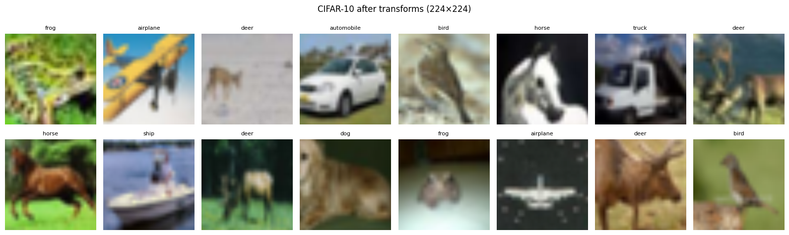
Source
# ── Normalization: before vs after ──────────────────────────────────────────
# Show how the same image looks as a raw tensor, as a normalized tensor,
# and after denormalization — so students understand WHY denormalize() is needed.

# Build a separate pipeline WITHOUT normalization (just resize + crop + ToTensor)
raw_transform = transforms.Compose([
    transforms.Resize(RESIZE_SIZE),
    transforms.CenterCrop(TRAIN_IMAGE_SIZE),
    transforms.ToTensor(),          # values in [0, 1], no mean/std shift
])
raw_dataset = datasets.CIFAR10(root='./data', train=False, download=False,
                                transform=raw_transform)
raw_img = raw_dataset[0][0]           # shape [3, H, W], values in [0, 1]

# Apply normalization manually to get the "model-ready" version
norm_fn  = transforms.Normalize(IMAGENET_MEAN, IMAGENET_STD)
norm_img = norm_fn(raw_img.clone())   # values now span roughly [-2.1, 2.6]

denorm_img = denormalize(norm_img)    # should reconstruct raw_img closely

fig, axes = plt.subplots(1, 3, figsize=(14, 4))

axes[0].imshow(raw_img.permute(1, 2, 0).numpy())
axes[0].set_title('① Raw image\n(values 0–1, looks normal)', fontsize=10)
axes[0].axis('off')

# Clip to show what matplotlib does without denormalization
axes[1].imshow(norm_img.permute(1, 2, 0).clamp(0, 1).numpy())
axes[1].set_title('② After ImageNet normalization\n(matplotlib clips values — colours distorted!)', fontsize=10)
axes[1].axis('off')

axes[2].imshow(denorm_img.permute(1, 2, 0).numpy())
axes[2].set_title('③ After denormalization\n(values restored — looks correct again)', fontsize=10)
axes[2].axis('off')

plt.suptitle(
    'Why we need denormalize() for display\n'
    'The model always receives ② — normalization stays on during training.\n'
    'We only apply denormalize() when showing images to humans.',
    fontsize=11
)
plt.tight_layout()
plt.show()

# Also show the pixel value histogram to make the range visible
fig, ax = plt.subplots(figsize=(9, 3))
ax.hist(raw_img.numpy().flatten(),  bins=60, alpha=0.6, label='Raw [0, 1]',         color='green')
ax.hist(norm_img.numpy().flatten(), bins=60, alpha=0.6, label='Normalized [~-2, 2]', color='blue')
ax.axvline(0, color='black', linestyle='--', linewidth=1.2, label='Display clip at 0')
ax.axvline(1, color='red',   linestyle='--', linewidth=1.2, label='Display clip at 1')
ax.set_xlabel('Pixel value')
ax.set_ylabel('Number of pixels')
ax.set_title('Pixel value distributions — normalization pushes values outside [0, 1]')
ax.legend(fontsize=9)
ax.grid(True, alpha=0.3)
plt.tight_layout()
plt.show()
print("Notice: ~half of the normalized pixels are below 0 — matplotlib clips these to black,")
print("which is why the clipped image ② looks dark and washed-out.")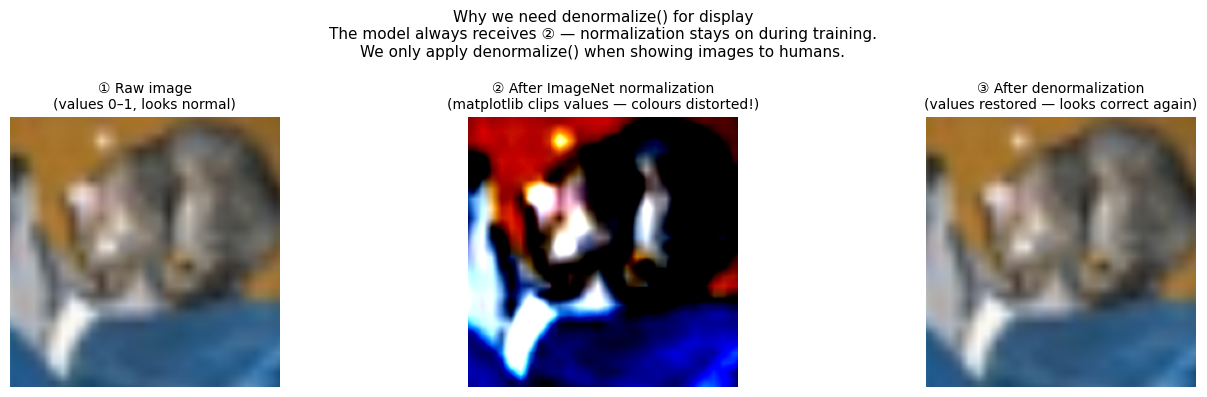
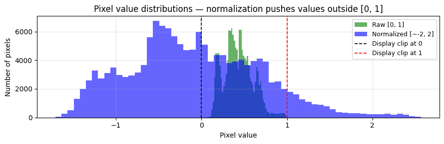
Notice: ~half of the normalized pixels are below 0 — matplotlib clips these to black,
which is why the clipped image ② looks dark and washed-out.
Part 3 — AlexNet Architecture (~10 min)
A Brief History
AlexNet (Krizhevsky, Sutskever, Hinton, 2012) won the ImageNet Large Scale Visual Recognition Challenge (ILSVRC) by a massive margin — top-5 error of 15.3% vs the runner-up’s 26.2%. It sparked the modern deep learning revolution.
Key innovations at the time:
First deep CNN to win ImageNet
Used ReLU activations (faster training than sigmoid/tanh)
Used Dropout in the classifier (reduced overfitting)
Trained on GPUs (allowed much faster training)
AlexNet Architecture
AlexNet has two logical sections:
Input: 3 × 224 × 224

features (5 conv blocks):
  Conv(3→64, k=11, s=4, p=2) → ReLU → MaxPool(3,2)    → 64×27×27
  Conv(64→192, k=5, p=2)     → ReLU → MaxPool(3,2)    → 192×13×13
  Conv(192→384, k=3, p=1)    → ReLU                   → 384×13×13
  Conv(384→256, k=3, p=1)    → ReLU                   → 256×13×13
  Conv(256→256, k=3, p=1)    → ReLU → MaxPool(3,2)    → 256×6×6

avgpool → 256×6×6

classifier (3 FC layers):
  Dropout → Linear(9216→4096) → ReLU
  Dropout → Linear(4096→4096) → ReLU
           → Linear(4096→1000)           ← we replace this!
The classifier[6] layer is the final Linear(4096→1000). We replace it with Linear(4096→10).
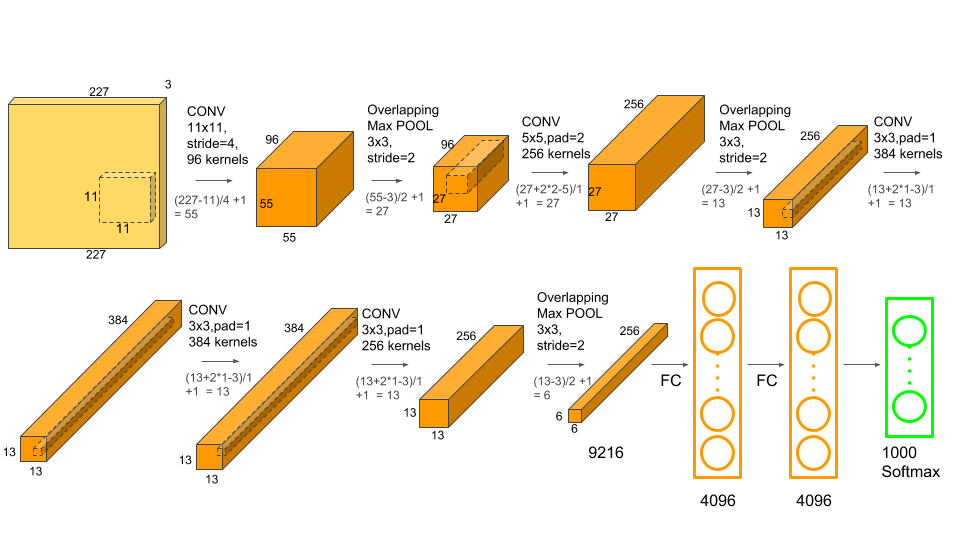
AlexNet architecture: 5 convolutional layers followed by 3 fully-connected layers. The first conv uses large 11×11 kernels with stride 4; subsequent layers use smaller 5×5 and 3×3 kernels. Max pooling appears after the 1st, 2nd, and 5th conv layers. The classifier (classifier[6], shown as the last FC) outputs 1000 ImageNet class scores — this is the layer we replace with Linear(4096→10) for CIFAR-10.
AlexNet has two key sub-modules:
.features— all convolutional layers (the backbone we will freeze).classifier— the fully-connected head (we will replace the last layer:classifier[6])
Note:
weights=AlexNet_Weights.DEFAULTdownloads the best available ImageNet checkpoint. The first run will download ~233 MB (cached in~/.cache/torch/hub/checkpoints/).
alexnet_raw = models.alexnet(weights=AlexNet_Weights.DEFAULT)
print(alexnet_raw)

print('\n--- features ---')
for i, layer in enumerate(alexnet_raw.features):
    print(f'  features[{i}]: {layer}')

print('\n--- classifier ---')
for i, layer in enumerate(alexnet_raw.classifier):
    print(f'  classifier[{i}]: {layer}')

print(f'\nclassifier[6] is the layer we will replace: {alexnet_raw.classifier[6]}')
AlexNet(
(features): Sequential(
(0): Conv2d(3, 64, kernel_size=(11, 11), stride=(4, 4), padding=(2, 2))
(1): ReLU(inplace=True)
(2): MaxPool2d(kernel_size=3, stride=2, padding=0, dilation=1, ceil_mode=False)
(3): Conv2d(64, 192, kernel_size=(5, 5), stride=(1, 1), padding=(2, 2))
(4): ReLU(inplace=True)
(5): MaxPool2d(kernel_size=3, stride=2, padding=0, dilation=1, ceil_mode=False)
(6): Conv2d(192, 384, kernel_size=(3, 3), stride=(1, 1), padding=(1, 1))
(7): ReLU(inplace=True)
(8): Conv2d(384, 256, kernel_size=(3, 3), stride=(1, 1), padding=(1, 1))
(9): ReLU(inplace=True)
(10): Conv2d(256, 256, kernel_size=(3, 3), stride=(1, 1), padding=(1, 1))
(11): ReLU(inplace=True)
(12): MaxPool2d(kernel_size=3, stride=2, padding=0, dilation=1, ceil_mode=False)
)
(avgpool): AdaptiveAvgPool2d(output_size=(6, 6))
(classifier): Sequential(
(0): Dropout(p=0.5, inplace=False)
(1): Linear(in_features=9216, out_features=4096, bias=True)
(2): ReLU(inplace=True)
(3): Dropout(p=0.5, inplace=False)
(4): Linear(in_features=4096, out_features=4096, bias=True)
(5): ReLU(inplace=True)
(6): Linear(in_features=4096, out_features=1000, bias=True)
)
)
--- features ---
features[0]: Conv2d(3, 64, kernel_size=(11, 11), stride=(4, 4), padding=(2, 2))
features[1]: ReLU(inplace=True)
features[2]: MaxPool2d(kernel_size=3, stride=2, padding=0, dilation=1, ceil_mode=False)
features[3]: Conv2d(64, 192, kernel_size=(5, 5), stride=(1, 1), padding=(2, 2))
features[4]: ReLU(inplace=True)
features[5]: MaxPool2d(kernel_size=3, stride=2, padding=0, dilation=1, ceil_mode=False)
features[6]: Conv2d(192, 384, kernel_size=(3, 3), stride=(1, 1), padding=(1, 1))
features[7]: ReLU(inplace=True)
features[8]: Conv2d(384, 256, kernel_size=(3, 3), stride=(1, 1), padding=(1, 1))
features[9]: ReLU(inplace=True)
features[10]: Conv2d(256, 256, kernel_size=(3, 3), stride=(1, 1), padding=(1, 1))
features[11]: ReLU(inplace=True)
features[12]: MaxPool2d(kernel_size=3, stride=2, padding=0, dilation=1, ceil_mode=False)
--- classifier ---
classifier[0]: Dropout(p=0.5, inplace=False)
classifier[1]: Linear(in_features=9216, out_features=4096, bias=True)
classifier[2]: ReLU(inplace=True)
classifier[3]: Dropout(p=0.5, inplace=False)
classifier[4]: Linear(in_features=4096, out_features=4096, bias=True)
classifier[5]: ReLU(inplace=True)
classifier[6]: Linear(in_features=4096, out_features=1000, bias=True)
classifier[6] is the layer we will replace: Linear(in_features=4096, out_features=1000, bias=True)
What Did AlexNet Learn to Look For?
We claimed that early CNN layers learn universal visual features — edges, colours, textures. Let’s verify that by looking directly at the weights of AlexNet’s first convolutional layer.
The first layer has 64 filters, each 11×11 pixels with 3 colour channels. Each filter is essentially a tiny template that the network slides over the image to detect a particular pattern. When you run the cell below, look for:
Diagonal edge detectors (bright-to-dark gradients at different angles)
Colour-opponent filters (one half red, other half green — detects colour contrast)
Blob detectors (bright centre, dark surround, or vice versa)
These patterns are not specific to ImageNet — they would look similar if you trained the network on any large collection of natural photographs. That is the core argument for why transfer learning works.
Source
# ── Visualise the 64 first-layer filters of AlexNet ─────────────────────────
weights = alexnet_raw.features[0].weight.data.clone()   # shape: [64, 3, 11, 11]

# Normalise each filter independently to [0, 1] for display
w_min = weights.view(64, -1).min(dim=1)[0].view(64, 1, 1, 1)
w_max = weights.view(64, -1).max(dim=1)[0].view(64, 1, 1, 1)
weights_norm = (weights - w_min) / (w_max - w_min + 1e-8)

fig, axes = plt.subplots(8, 8, figsize=(10, 10))
fig.suptitle(
    'AlexNet — 64 learned filters from the first convolutional layer (11×11 px, RGB)\n'
    'Look for: diagonal edges, colour gradients, orientation detectors — all universal patterns.',
    fontsize=10, y=1.02
)
for i, ax in enumerate(axes.ravel()):
    ax.imshow(weights_norm[i].permute(1, 2, 0).numpy())
    ax.axis('off')
plt.tight_layout()
plt.show()
print("These filters were learned from 1.2 million ImageNet photos.")
print("They are the patterns AlexNet detects in any image it processes — including our CIFAR-10 images.")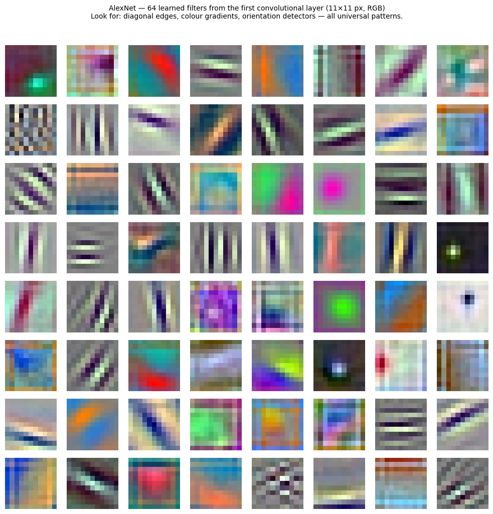
These filters were learned from 1.2 million ImageNet photos.
They are the patterns AlexNet detects in any image it processes — including our CIFAR-10 images.
Part 4 — AlexNet Transfer Learning: Step by Step (~25 min)
We now walk through each step of the transfer learning pipeline in detail.
The 5 Steps
Load model with pre-trained weights
Freeze all backbone parameters
Replace the final classifier layer
Unfreeze the new head and move model to GPU
Train only the new head
Let’s do each step one cell at a time, with a clear explanation of what and why.
# weights=AlexNet_Weights.DEFAULT is the modern API (old: pretrained=True, now deprecated).
# The model is cached in ~/.cache/torch/hub/checkpoints/ after the first download.
alexnet = models.alexnet(weights=AlexNet_Weights.DEFAULT)
print('AlexNet loaded with ImageNet weights.')
AlexNet loaded with ImageNet weights.
The requires_grad Flag
Every PyTorch parameter has a .requires_grad flag:
True→ PyTorch tracks gradients and the optimizer will update this parameterFalse→ PyTorch skips gradient computation entirely, saving memory and compute
We set all parameters to False first (freezing the entire network), then in Step 3
the new head we assign will have requires_grad=True by default.
for param in alexnet.parameters():
    param.requires_grad = False

trainable = sum(p.numel() for p in alexnet.parameters() if p.requires_grad)
print(f'Trainable parameters after freezing: {trainable:,}   (should be 0)')
Trainable parameters after freezing: 0 (should be 0)
✅ What just happened?
You should see:Trainable parameters after freezing: 0
This means PyTorch will not compute gradients for any layer — the entire network is locked.
We froze everything on purpose. In the next step we’ll replace the final layer, which will automatically become trainable again because newnn.Linearlayers haverequires_grad=Trueby default.
If you see a number other than 0 here, double-check that the loop ran before you re-used the variable name.
Why Replace classifier[6]?
The original AlexNet classifier has this structure:
| Index | Layer |
|---|---|
[0] | Dropout |
[1] | Linear(9216, 4096) |
[2] | ReLU |
[3] | Dropout |
[4] | Linear(4096, 4096) |
[5] | ReLU |
[6] | Linear(4096, 1000) ← replace this |
We swap classifier[6] with Linear(4096, 10) — keeping 4096 input features but
reducing the output from 1000 ImageNet classes to 10 CIFAR-10 classes.
The new layer gets requires_grad=True by default.
alexnet.classifier[6] = nn.Linear(4096, 10)

print(f'New output layer: {alexnet.classifier[6]}')
print(f'Its requires_grad: {alexnet.classifier[6].weight.requires_grad}')

# Explicitly ensure the new layer's parameters are trainable
for param in alexnet.classifier[6].parameters():
    param.requires_grad = True
New output layer: Linear(in_features=4096, out_features=10, bias=True)
Its requires_grad: True
Move to Device and Sanity-Check
After replacing the classifier, we move the full model to the selected device.
A quick dummy forward pass confirms the output shape is [batch_size, 10].
alexnet = alexnet.to(device)

total_params     = sum(p.numel() for p in alexnet.parameters())
trainable_params = sum(p.numel() for p in alexnet.parameters() if p.requires_grad)
frozen_params    = total_params - trainable_params

print('=' * 55)
print(f"{'Total parameters':<30} {total_params:>15,}")
print(f"{'Frozen parameters':<30} {frozen_params:>15,}")
print(f"{'Trainable parameters':<30} {trainable_params:>15,}")
print(f"{'Fraction trainable':<30} {100.*trainable_params/total_params:>14.2f}%")
print('=' * 55)

with torch.no_grad():
    dummy_in  = torch.zeros(2, 3, TRAIN_IMAGE_SIZE, TRAIN_IMAGE_SIZE).to(device)
    dummy_out = alexnet(dummy_in)
print(f'\nOutput shape for a batch of 2: {dummy_out.shape}   (expected: [2, 10])')
=======================================================
Total parameters 57,044,810
Frozen parameters 57,003,840
Trainable parameters 40,970
Fraction trainable 0.07%
=======================================================
Output shape for a batch of 2: torch.Size([2, 10]) (expected: [2, 10])
✅ What just happened?
You should see something like:Total parameters 61,100,840 Frozen parameters 61,059,840 Trainable parameters 41,000 Fraction trainable 0.07%That means only ~41,000 parameters (the new
Linear(4096→10)layer) will be updated during training. The other 61 million are locked.The dummy forward pass should print
Output shape for a batch of 2: torch.Size([2, 10]).
If you see[2, 1000], the layer replacement step did not run — go back and run cell Step 3 again.
Step 5: Defining the Optimiser, Loss, and Scheduler
Three important decisions:
Loss function — CrossEntropyLoss
Standard choice for multi-class classification. Combines LogSoftmax + NLLLoss in one numerically stable operation.
Optimiser — Adam with only the trainable params
We pass filter(lambda p: p.requires_grad, ...) so the optimiser only tracks the new head.
Why does this matter?
Frozen parameters won’t receive gradient updates anyway, but including them in the optimiser wastes memory (Adam stores a moving average for every parameter it tracks).
Passing only trainable params keeps the optimiser state small and fast.
Think before the next cell: What do you think would happen to memory usage if you accidentally passed all of AlexNet’s 61 million parameters to Adam instead of just the trainable 41,000? Keep your answer in mind — Q3 after the training cell will ask exactly this.
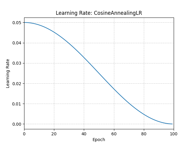
Scheduler — CosineAnnealingLR
Instead of using a fixed learning rate for all epochs, the scheduler decreases the LR following
a cosine curve from lr=1e-3 down to nearly 0 over T_max epochs.
Analogy: Think of parallel parking. You start with a big move to get close to the curb, then smaller and smaller nudges until you’re perfectly in place. Training works the same way: large learning rate early (find the right ballpark), then tiny adjustments at the end (fine-tune precisely). The cosine shape just means the transition is smooth rather than sudden.
# These helpers are reusable — we call them for both AlexNet and ResNet18.

def train_epoch(model, loader, criterion, optimizer, device):
    """Run one full pass over the training set. Returns (avg_loss, accuracy %)."""
    model.train()
    # Accumulate on device to avoid frequent synchronization
    total_loss = torch.tensor(0.0, device=device)
    correct = torch.tensor(0, device=device)
    total = 0

    for images, labels in loader:
        images, labels = images.to(device), labels.to(device)

        optimizer.zero_grad()
        outputs = model(images)
        loss = criterion(outputs, labels)
        loss.backward()
        optimizer.step()

        total_loss += loss.detach() * images.size(0)
        _, predicted = outputs.max(1)
        correct += predicted.eq(labels).sum()
        total   += labels.size(0)

    # Move to CPU only once at the end of the epoch
    return total_loss.item() / total, 100.0 * correct.item() / total


def evaluate(model, loader, criterion, device):
    """Evaluate the model on a dataset. Returns (avg_loss, accuracy %)."""
    model.eval()
    total_loss = torch.tensor(0.0, device=device)
    correct = torch.tensor(0, device=device)
    total = 0

    with torch.no_grad():
        for images, labels in loader:
            images, labels = images.to(device), labels.to(device)
            outputs = model(images)
            loss = criterion(outputs, labels)
            total_loss += loss * images.size(0)
            _, predicted = outputs.max(1)
            correct += predicted.eq(labels).sum()
            total   += labels.size(0)

    return total_loss.item() / total, 100.0 * correct.item() / total

print('Training utilities defined.')
Training utilities defined.
NUM_EPOCHS = 2

criterion = nn.CrossEntropyLoss()

# Only pass parameters that require gradients (the new 4096→10 head)
optimizer = optim.Adam(
    filter(lambda p: p.requires_grad, alexnet.parameters()),
    lr=1e-3,
    weight_decay=5e-4   # L2 regularisation to prevent overfitting of the small head
)

# Cosine annealing: smoothly reduces LR from 1e-3 to ~0 over NUM_EPOCHS
scheduler = optim.lr_scheduler.CosineAnnealingLR(optimizer, T_max=NUM_EPOCHS)

alexnet_history = {'train_loss': [], 'val_loss': [], 'train_acc': [], 'val_acc': []}

print(f'Fine-tuning AlexNet on CIFAR-10 for {NUM_EPOCHS} epochs ...')
print(f"{'Epoch':>5} | {'Train Loss':>10} | {'Train Acc':>9} | {'Val Loss':>8} | {'Val Acc':>7} | {'LR':>8}")
print('-' * 62)

for epoch in range(NUM_EPOCHS):
    current_lr = optimizer.param_groups[0]['lr']

    tr_loss, tr_acc = train_epoch(alexnet, train_loader, criterion, optimizer, device)
    va_loss, va_acc = evaluate(alexnet, test_loader, criterion, device)

    scheduler.step()   # adjusts LR for the next epoch

    alexnet_history['train_loss'].append(tr_loss)
    alexnet_history['val_loss'].append(va_loss)
    alexnet_history['train_acc'].append(tr_acc)
    alexnet_history['val_acc'].append(va_acc)

    print(f'{epoch+1:>5} | {tr_loss:>10.4f} | {tr_acc:>8.2f}% | {va_loss:>8.4f} | {va_acc:>6.2f}% | {current_lr:>8.6f}')

print(f'\nFinal AlexNet test accuracy: {alexnet_history["val_acc"][-1]:.2f}%')
Fine-tuning AlexNet on CIFAR-10 for 2 epochs ...
Epoch | Train Loss | Train Acc | Val Loss | Val Acc | LR
--------------------------------------------------------------
1 | 0.7971 | 71.92% | 0.5890 | 79.29% | 0.001000
2 | 0.6642 | 76.80% | 0.5348 | 81.07% | 0.000500
Final AlexNet test accuracy: 81.07%
✅ What to expect after training
With a frozen backbone and only 2 epochs, you should see roughly:
Train accuracy: ~50–65%
Validation accuracy: ~50–65%
This might sound modest, but remember:
Random guessing on 10 classes gives 10% accuracy.
We are training only ~41,000 parameters for 2 epochs — the backbone does all the heavy lifting.
Training more epochs (5–10) with an unfrozen head usually reaches 70–80%.
If your validation accuracy is stuck below 20%, go back and check that (1) the freeze step ran, (2) the layer replacement step ran, and (3) you’re using ImageNet normalization.
# ── Plot AlexNet training curves ──────────────────────────────────────
epochs = range(1, NUM_EPOCHS + 1)
fig, (ax1, ax2) = plt.subplots(1, 2, figsize=(13, 4))

ax1.plot(epochs, alexnet_history['train_loss'], 'b-o', label='Train Loss', markersize=5)
ax1.plot(epochs, alexnet_history['val_loss'],   'r-s', label='Val Loss',   markersize=5)
ax1.set_xlabel('Epoch')
ax1.set_ylabel('Loss')
ax1.set_title('AlexNet — Loss Curves')
ax1.legend()
ax1.grid(True, alpha=0.3)

ax2.plot(epochs, alexnet_history['train_acc'], 'b-o', label='Train Acc', markersize=5)
ax2.plot(epochs, alexnet_history['val_acc'],   'r-s', label='Val Acc',   markersize=5)
ax2.set_xlabel('Epoch')
ax2.set_ylabel('Accuracy (%)')
ax2.set_title('AlexNet — Accuracy Curves')
ax2.legend()
ax2.grid(True, alpha=0.3)

plt.tight_layout()
plt.show()

print(f'AlexNet reached {alexnet_history["val_acc"][-1]:.2f}% test accuracy '
      f'after {NUM_EPOCHS} epochs of fine-tuning.')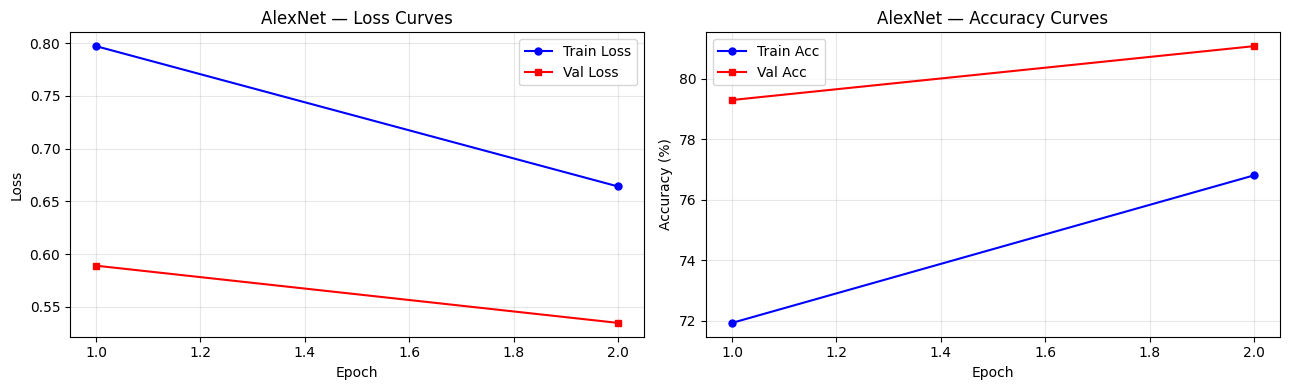
AlexNet reached 81.07% test accuracy after 2 epochs of fine-tuning.
✅ Check Your Understanding — AlexNet
Q3: We pass filter(lambda p: p.requires_grad, alexnet.parameters()) to the optimizer. What is the effect if we accidentally passed ALL parameters instead?
A) No difference — the optimizer would skip frozen params automatically
B) Higher memory usage (optimizer would maintain state for all 61M params) and minor risk of accidentally updating frozen layers if their grad flags change
C) A runtime error — PyTorch does not allow mixing frozen and unfrozen params
D) The model would train faster
Click to reveal solution
Answer: B)
Frozen parameters (requires_grad=False) will not receive gradient updates regardless.
However, optimisers like Adam maintain a running mean and variance for every parameter they track.
Passing all 61M parameters wastes memory — AlexNet’s ~60M frozen params would each get their own Adam state tensors, even though they’ll never be updated.
Q4: Why do we call model.train() at the start of each training epoch and model.eval() during evaluation?
A) It’s optional — just a convention
B)
model.train()enables Dropout and batch-wise BatchNorm stats;model.eval()disables Dropout and uses stored running stats — both affect the outputC)
model.train()moves the model to GPU;model.eval()moves it back to CPUD)
model.eval()freezes all layers permanently
Click to reveal solution
Answer: B)
AlexNet uses Dropout in its classifier. During training (model.train()), Dropout randomly zeros some neurons — this is intentional regularisation. During evaluation (model.eval()), we want deterministic, full predictions, so Dropout is turned off. Getting this wrong can cause validation accuracy to appear lower than it actually is.
🛑 Mid-Tutorial Checkpoint
Before moving on to ResNet18, make sure you can answer all three of these from memory:
Why do we freeze the backbone?
(Hint: think about what catastrophic forgetting means.)Which specific layer did we replace in AlexNet, and what was the input/output size before and after?
(Hint:classifier[6]:Linear(4096, ???)→Linear(4096, ???))How many parameters are actually being trained?
(Hint: ~41,000 — the frozen backbone has ~61 million, but we don’t touch those.)
If you’re unsure about any of these, scroll back and re-read the relevant section before continuing. ResNet18 uses the exact same 5-step recipe — understanding it well now means the next section will be fast.
Part 5 — ResNet18 Architecture (~10 min)
From Plain CNNs to Residual Learning (2015)
By 2015, CNNs kept getting deeper, but very deep plain networks became harder to optimise. The ResNet family (He et al.) introduced a simple but powerful idea: skip connections.
Instead of asking a stack of layers to learn a full transformation H(x), ResNet asks it to learn
only the residual part F(x) = H(x) - x, then adds the original input back:
out = F(x) + xThis makes gradient flow easier, lets deeper networks train more reliably, and became one of the most influential ideas in computer vision.
Why Skip Connections Matter
A residual block has two paths:
Main path: a few convolutional layers that learn
F(x)Skip path: the input
x, passed forward unchanged (or projected if shapes change)
If the new layers are not useful yet, the block can behave almost like the identity function. That makes optimisation much more stable than forcing every stack of layers to learn from scratch.
ResNet18 Architecture (Data Flow)
Compare this with the AlexNet diagram from Part 3:
Input: 3 × 224 × 224

Stem:
  Conv(3→64, k=7, s=2, p=3) → BatchNorm → ReLU → MaxPool(3, s=2)  → 64 × 56 × 56

layer1  (2 × BasicBlock, 64 ch):
  ┌─ Conv(64→64, k=3) → BN → ReLU → Conv(64→64, k=3) → BN ─┐
  └────────────────── skip: identity ───────────────────────┘
  → add → ReLU                                              → 64 × 56 × 56

layer2  (2 × BasicBlock, 128 ch, ×2 downsample):
  ┌─ Conv(64→128, k=3, s=2) → BN → ReLU → Conv(128→128) → BN ─┐
  └─────────────── skip: Conv(64→128, s=2) ────────────────────┘
  → add → ReLU                                              → 128 × 28 × 28

layer3  (2 × BasicBlock, 256 ch, ×2 downsample):          → 256 × 14 × 14
layer4  (2 × BasicBlock, 512 ch, ×2 downsample):          → 512 ×  7 ×  7

avgpool (global average pool):                             → 512 × 1 × 1
flatten:                                                   → 512
fc:  Linear(512 → 1000)    ← we replace with Linear(512 → 10)
Key difference from AlexNet:
No large fully-connected head (
4096 → 4096 → 1000); just oneLinear(512 → 10)Much fewer trainable parameters when we freeze the backbone
Deeper network but more parameter-efficient
ResNet18 has these key sub-modules:
conv1+maxpool— the stem that quickly expands channels and reduces spatial sizelayer1...layer4— four stages of residual blocksavgpool— global average pooling down to one feature vector per imagefc— the final linear classifier we replace for CIFAR-10
Note:
weights=ResNet18_Weights.DEFAULTdownloads a much smaller checkpoint than many older CNN checkpoints (about 45 MB), so the first run is usually quicker.
Source
# ── ResNet18 spatial size and channel count through the network ──────────────
stages     = ['Input', 'After Stem', 'layer1', 'layer2', 'layer3', 'layer4', 'After\navgpool']
channels   = [3,        64,           64,       128,      256,      512,      512]
spatial    = [224,      56,           56,        28,       14,        7,        1]

fig, (ax1, ax2) = plt.subplots(1, 2, figsize=(12, 4))

# Channel count grows as we go deeper
bars1 = ax1.bar(stages, channels, color=['#4CAF50','#2196F3','#2196F3','#1976D2','#1565C0','#0D47A1','#FF5722'])
ax1.set_ylabel('Number of channels')
ax1.set_title('ResNet18: Channel count per stage\n(gets wider as it gets deeper)')
ax1.set_ylim(0, 580)
for bar, val in zip(bars1, channels):
    ax1.text(bar.get_x() + bar.get_width()/2, bar.get_height() + 8,
             str(val), ha='center', va='bottom', fontsize=9, fontweight='bold')
ax1.tick_params(axis='x', labelrotation=15)
ax1.grid(True, alpha=0.3, axis='y')

# Spatial size shrinks as we go deeper
bars2 = ax2.bar(stages, spatial, color=['#4CAF50','#FF9800','#FF9800','#F57C00','#E65100','#BF360C','#FF5722'])
ax2.set_ylabel('Spatial size (one side, pixels)')
ax2.set_title('ResNet18: Feature map size per stage\n(gets smaller as it gets deeper)')
ax2.set_ylim(0, 250)
for bar, val in zip(bars2, spatial):
    ax2.text(bar.get_x() + bar.get_width()/2, bar.get_height() + 3,
             f'{val}×{val}', ha='center', va='bottom', fontsize=9, fontweight='bold')
ax2.tick_params(axis='x', labelrotation=15)
ax2.grid(True, alpha=0.3, axis='y')

plt.suptitle('As ResNet18 processes an image: channels grow, spatial size shrinks.\n'
             'The network trades spatial detail for richer feature descriptions.',
             fontsize=10)
plt.tight_layout()
plt.show()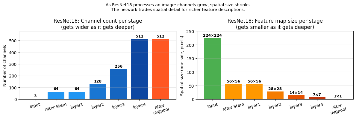
ResNet18 has a different internal structure from AlexNet:
No
.features/.classifiersplitInstead:
conv1→bn1→relu→maxpool→layer1–layer4→avgpool→fcThe final classifier is a single
fclayer, not a 3-layer MLP like AlexNet
Note:
weights=ResNet18_Weights.DEFAULTdownloads a checkpoint of about 45 MB — much smaller than many older CNN checkpoints. The first run will download it to~/.cache/torch/hub/checkpoints/. Subsequent runs use the cached file and are instant.
resnet_raw = models.resnet18(weights=ResNet18_Weights.DEFAULT)
print(resnet_raw)

print('\n--- top-level modules ---')
for name, module in resnet_raw.named_children():
    print(f'  {name}: {module}')
Downloading: "https://download.pytorch.org/models/resnet18-f37072fd.pth" to /Users/lnguyen/.cache/torch/hub/checkpoints/resnet18-f37072fd.pth
100%|██████████| 44.7M/44.7M [00:04<00:00, 11.5MB/s]
ResNet(
  (conv1): Conv2d(3, 64, kernel_size=(7, 7), stride=(2, 2), padding=(3, 3), bias=False)
  (bn1): BatchNorm2d(64, eps=1e-05, momentum=0.1, affine=True, track_running_stats=True)
  (relu): ReLU(inplace=True)
  (maxpool): MaxPool2d(kernel_size=3, stride=2, padding=1, dilation=1, ceil_mode=False)
  (layer1): Sequential(
    (0): BasicBlock(
      (conv1): Conv2d(64, 64, kernel_size=(3, 3), stride=(1, 1), padding=(1, 1), bias=False)
      (bn1): BatchNorm2d(64, eps=1e-05, momentum=0.1, affine=True, track_running_stats=True)
      (relu): ReLU(inplace=True)
      (conv2): Conv2d(64, 64, kernel_size=(3, 3), stride=(1, 1), padding=(1, 1), bias=False)
      (bn2): BatchNorm2d(64, eps=1e-05, momentum=0.1, affine=True, track_running_stats=True)
    )
    (1): BasicBlock(
      (conv1): Conv2d(64, 64, kernel_size=(3, 3), stride=(1, 1), padding=(1, 1), bias=False)
      (bn1): BatchNorm2d(64, eps=1e-05, momentum=0.1, affine=True, track_running_stats=True)
      (relu): ReLU(inplace=True)
      (conv2): Conv2d(64, 64, kernel_size=(3, 3), stride=(1, 1), padding=(1, 1), bias=False)
      (bn2): BatchNorm2d(64, eps=1e-05, momentum=0.1, affine=True, track_running_stats=True)
    )
  )
  (layer2): Sequential(
    (0): BasicBlock(
      (conv1): Conv2d(64, 128, kernel_size=(3, 3), stride=(2, 2), padding=(1, 1), bias=False)
      (bn1): BatchNorm2d(128, eps=1e-05, momentum=0.1, affine=True, track_running_stats=True)
      (relu): ReLU(inplace=True)
      (conv2): Conv2d(128, 128, kernel_size=(3, 3), stride=(1, 1), padding=(1, 1), bias=False)
      (bn2): BatchNorm2d(128, eps=1e-05, momentum=0.1, affine=True, track_running_stats=True)
      (downsample): Sequential(
        (0): Conv2d(64, 128, kernel_size=(1, 1), stride=(2, 2), bias=False)
        (1): BatchNorm2d(128, eps=1e-05, momentum=0.1, affine=True, track_running_stats=True)
      )
    )
    (1): BasicBlock(
      (conv1): Conv2d(128, 128, kernel_size=(3, 3), stride=(1, 1), padding=(1, 1), bias=False)
      (bn1): BatchNorm2d(128, eps=1e-05, momentum=0.1, affine=True, track_running_stats=True)
      (relu): ReLU(inplace=True)
      (conv2): Conv2d(128, 128, kernel_size=(3, 3), stride=(1, 1), padding=(1, 1), bias=False)
      (bn2): BatchNorm2d(128, eps=1e-05, momentum=0.1, affine=True, track_running_stats=True)
    )
  )
  (layer3): Sequential(
    (0): BasicBlock(
      (conv1): Conv2d(128, 256, kernel_size=(3, 3), stride=(2, 2), padding=(1, 1), bias=False)
      (bn1): BatchNorm2d(256, eps=1e-05, momentum=0.1, affine=True, track_running_stats=True)
      (relu): ReLU(inplace=True)
      (conv2): Conv2d(256, 256, kernel_size=(3, 3), stride=(1, 1), padding=(1, 1), bias=False)
      (bn2): BatchNorm2d(256, eps=1e-05, momentum=0.1, affine=True, track_running_stats=True)
      (downsample): Sequential(
        (0): Conv2d(128, 256, kernel_size=(1, 1), stride=(2, 2), bias=False)
        (1): BatchNorm2d(256, eps=1e-05, momentum=0.1, affine=True, track_running_stats=True)
      )
    )
    (1): BasicBlock(
      (conv1): Conv2d(256, 256, kernel_size=(3, 3), stride=(1, 1), padding=(1, 1), bias=False)
      (bn1): BatchNorm2d(256, eps=1e-05, momentum=0.1, affine=True, track_running_stats=True)
      (relu): ReLU(inplace=True)
      (conv2): Conv2d(256, 256, kernel_size=(3, 3), stride=(1, 1), padding=(1, 1), bias=False)
      (bn2): BatchNorm2d(256, eps=1e-05, momentum=0.1, affine=True, track_running_stats=True)
    )
  )
  (layer4): Sequential(
    (0): BasicBlock(
      (conv1): Conv2d(256, 512, kernel_size=(3, 3), stride=(2, 2), padding=(1, 1), bias=False)
      (bn1): BatchNorm2d(512, eps=1e-05, momentum=0.1, affine=True, track_running_stats=True)
      (relu): ReLU(inplace=True)
      (conv2): Conv2d(512, 512, kernel_size=(3, 3), stride=(1, 1), padding=(1, 1), bias=False)
      (bn2): BatchNorm2d(512, eps=1e-05, momentum=0.1, affine=True, track_running_stats=True)
      (downsample): Sequential(
        (0): Conv2d(256, 512, kernel_size=(1, 1), stride=(2, 2), bias=False)
        (1): BatchNorm2d(512, eps=1e-05, momentum=0.1, affine=True, track_running_stats=True)
      )
    )
    (1): BasicBlock(
      (conv1): Conv2d(512, 512, kernel_size=(3, 3), stride=(1, 1), padding=(1, 1), bias=False)
      (bn1): BatchNorm2d(512, eps=1e-05, momentum=0.1, affine=True, track_running_stats=True)
      (relu): ReLU(inplace=True)
      (conv2): Conv2d(512, 512, kernel_size=(3, 3), stride=(1, 1), padding=(1, 1), bias=False)
      (bn2): BatchNorm2d(512, eps=1e-05, momentum=0.1, affine=True, track_running_stats=True)
    )
  )
  (avgpool): AdaptiveAvgPool2d(output_size=(1, 1))
  (fc): Linear(in_features=512, out_features=1000, bias=True)
)

--- top-level modules ---
  conv1: Conv2d(3, 64, kernel_size=(7, 7), stride=(2, 2), padding=(3, 3), bias=False)
  bn1: BatchNorm2d(64, eps=1e-05, momentum=0.1, affine=True, track_running_stats=True)
  relu: ReLU(inplace=True)
  maxpool: MaxPool2d(kernel_size=3, stride=2, padding=1, dilation=1, ceil_mode=False)
  layer1: Sequential(
  (0): BasicBlock(
    (conv1): Conv2d(64, 64, kernel_size=(3, 3), stride=(1, 1), padding=(1, 1), bias=False)
    (bn1): BatchNorm2d(64, eps=1e-05, momentum=0.1, affine=True, track_running_stats=True)
    (relu): ReLU(inplace=True)
    (conv2): Conv2d(64, 64, kernel_size=(3, 3), stride=(1, 1), padding=(1, 1), bias=False)
    (bn2): BatchNorm2d(64, eps=1e-05, momentum=0.1, affine=True, track_running_stats=True)
  )
  (1): BasicBlock(
    (conv1): Conv2d(64, 64, kernel_size=(3, 3), stride=(1, 1), padding=(1, 1), bias=False)
    (bn1): BatchNorm2d(64, eps=1e-05, momentum=0.1, affine=True, track_running_stats=True)
    (relu): ReLU(inplace=True)
    (conv2): Conv2d(64, 64, kernel_size=(3, 3), stride=(1, 1), padding=(1, 1), bias=False)
    (bn2): BatchNorm2d(64, eps=1e-05, momentum=0.1, affine=True, track_running_stats=True)
  )
)
  layer2: Sequential(
  (0): BasicBlock(
    (conv1): Conv2d(64, 128, kernel_size=(3, 3), stride=(2, 2), padding=(1, 1), bias=False)
    (bn1): BatchNorm2d(128, eps=1e-05, momentum=0.1, affine=True, track_running_stats=True)
    (relu): ReLU(inplace=True)
    (conv2): Conv2d(128, 128, kernel_size=(3, 3), stride=(1, 1), padding=(1, 1), bias=False)
    (bn2): BatchNorm2d(128, eps=1e-05, momentum=0.1, affine=True, track_running_stats=True)
    (downsample): Sequential(
      (0): Conv2d(64, 128, kernel_size=(1, 1), stride=(2, 2), bias=False)
      (1): BatchNorm2d(128, eps=1e-05, momentum=0.1, affine=True, track_running_stats=True)
    )
  )
  (1): BasicBlock(
    (conv1): Conv2d(128, 128, kernel_size=(3, 3), stride=(1, 1), padding=(1, 1), bias=False)
    (bn1): BatchNorm2d(128, eps=1e-05, momentum=0.1, affine=True, track_running_stats=True)
    (relu): ReLU(inplace=True)
    (conv2): Conv2d(128, 128, kernel_size=(3, 3), stride=(1, 1), padding=(1, 1), bias=False)
    (bn2): BatchNorm2d(128, eps=1e-05, momentum=0.1, affine=True, track_running_stats=True)
  )
)
  layer3: Sequential(
  (0): BasicBlock(
    (conv1): Conv2d(128, 256, kernel_size=(3, 3), stride=(2, 2), padding=(1, 1), bias=False)
    (bn1): BatchNorm2d(256, eps=1e-05, momentum=0.1, affine=True, track_running_stats=True)
    (relu): ReLU(inplace=True)
    (conv2): Conv2d(256, 256, kernel_size=(3, 3), stride=(1, 1), padding=(1, 1), bias=False)
    (bn2): BatchNorm2d(256, eps=1e-05, momentum=0.1, affine=True, track_running_stats=True)
    (downsample): Sequential(
      (0): Conv2d(128, 256, kernel_size=(1, 1), stride=(2, 2), bias=False)
      (1): BatchNorm2d(256, eps=1e-05, momentum=0.1, affine=True, track_running_stats=True)
    )
  )
  (1): BasicBlock(
    (conv1): Conv2d(256, 256, kernel_size=(3, 3), stride=(1, 1), padding=(1, 1), bias=False)
    (bn1): BatchNorm2d(256, eps=1e-05, momentum=0.1, affine=True, track_running_stats=True)
    (relu): ReLU(inplace=True)
    (conv2): Conv2d(256, 256, kernel_size=(3, 3), stride=(1, 1), padding=(1, 1), bias=False)
    (bn2): BatchNorm2d(256, eps=1e-05, momentum=0.1, affine=True, track_running_stats=True)
  )
)
  layer4: Sequential(
  (0): BasicBlock(
    (conv1): Conv2d(256, 512, kernel_size=(3, 3), stride=(2, 2), padding=(1, 1), bias=False)
    (bn1): BatchNorm2d(512, eps=1e-05, momentum=0.1, affine=True, track_running_stats=True)
    (relu): ReLU(inplace=True)
    (conv2): Conv2d(512, 512, kernel_size=(3, 3), stride=(1, 1), padding=(1, 1), bias=False)
    (bn2): BatchNorm2d(512, eps=1e-05, momentum=0.1, affine=True, track_running_stats=True)
    (downsample): Sequential(
      (0): Conv2d(256, 512, kernel_size=(1, 1), stride=(2, 2), bias=False)
      (1): BatchNorm2d(512, eps=1e-05, momentum=0.1, affine=True, track_running_stats=True)
    )
  )
  (1): BasicBlock(
    (conv1): Conv2d(512, 512, kernel_size=(3, 3), stride=(1, 1), padding=(1, 1), bias=False)
    (bn1): BatchNorm2d(512, eps=1e-05, momentum=0.1, affine=True, track_running_stats=True)
    (relu): ReLU(inplace=True)
    (conv2): Conv2d(512, 512, kernel_size=(3, 3), stride=(1, 1), padding=(1, 1), bias=False)
    (bn2): BatchNorm2d(512, eps=1e-05, momentum=0.1, affine=True, track_running_stats=True)
  )
)
  avgpool: AdaptiveAvgPool2d(output_size=(1, 1))
  fc: Linear(in_features=512, out_features=1000, bias=True)
How to Read the Printed Architecture
The output above shows ResNet18’s full structure. Here is what to look for:
Top-level modules (from named_children()):
conv1,bn1,relu,maxpool→ the stem (processes input, reduces spatial size fast)layer1...layer4→ four stages of BasicBlocks (the residual backbone)avgpool→ squashes512×7×7down to a single512-dim vectorfc→ the final classifier we replace:Linear(512, 1000)
Inside the BasicBlocks:
Each BasicBlock has:
conv1,bn1,relu,conv2,bn2→ the main path (learns the residual F(x))downsample→ only present when the spatial size or channel count changes (i.e. the skip path needs a projection)
What to replace: Only
resnet.fc— the very last line of the printed architecture. Everything above it stays frozen and untouched.
Understanding the Residual Block Pattern
ResNet18 is built from BasicBlock modules. Each block has two 3×3 convolutions plus a skip path.
| Stage | Output channels | Typical spatial size (from 224) | Notes |
|---|---|---|---|
| Stem | 64 | 56×56 | 7×7 conv + max pool |
layer1 | 64 | 56×56 | residual blocks, no downsampling |
layer2 | 128 | 28×28 | first block downsamples |
layer3 | 256 | 14×14 | first block downsamples |
layer4 | 512 | 7×7 | first block downsamples |
After the final stage, global average pooling reduces 512×7×7 to a length-512 vector.
That vector feeds the final fc layer, so transfer learning only needs to replace Linear(512→1000)
with Linear(512→10).
The Residual Idea
A simplified residual block looks like this:
input x
   │
   ├─────────────── skip connection ───────────────┐
   │                                               │
   └→ Conv → ReLU → Conv ──────────────────────────┤
                                                   ▼
                                             add: F(x) + x
                                                   │
                                                  ReLU
The addition is the key idea. Instead of rebuilding the entire representation every time, the block only learns how it should adjust the incoming features.
class ToyResidualBlock(nn.Module):
    # Minimal residual block for shape inspection.
    def __init__(self, channels):
        super().__init__()
        self.conv1 = nn.Conv2d(channels, channels, kernel_size=3, padding=1)
        self.relu = nn.ReLU(inplace=True)
        self.conv2 = nn.Conv2d(channels, channels, kernel_size=3, padding=1)

    def forward(self, x):
        identity = x
        out = self.conv1(x)
        out = self.relu(out)
        out = self.conv2(out)
        out = out + identity
        return self.relu(out)


x = torch.zeros(1, 64, 56, 56)
block = ToyResidualBlock(64)
with torch.no_grad():
    y = block(x)

print('Toy residual block shape trace:')
print(f'  input shape : {tuple(x.shape)}')
print(f'  output shape: {tuple(y.shape)}')
print('The shape stays the same, so the skip connection can be added elementwise.')
Toy residual block shape trace:
input shape : (1, 64, 56, 56)
output shape: (1, 64, 56, 56)
The shape stays the same, so the skip connection can be added elementwise.
Connecting the toy block to the real model
TheToyResidualBlockyou just ran is almost identical to what PyTorch calls aBasicBlockinside ResNet18. When you printresnet_rawin the next section, look for lines that sayBasicBlock(...)— those are 8 of these stacked acrosslayer1throughlayer4.The key thing to notice above: input shape equals output shape.
That is what makes theout = out + identityline work — you can only add two tensors elementwise if they have the same shape.
Part 6 — ResNet18 Transfer Learning: Step by Step (~20 min)
The transfer learning recipe is still almost identical to AlexNet:
Load with pretrained weights
Freeze all params
Replace
fcMove to device
Train only the head
The main architectural difference is that ResNet uses a single final fc layer after global average pooling,
so the head replacement is even smaller than AlexNet’s.
Step 1: Load ResNet18 with Pre-trained Weights
Same as AlexNet — pass weights=ResNet18_Weights.DEFAULT to get the ImageNet-trained version.
The checkpoint (~45 MB) is cached after the first download.
resnet = models.resnet18(weights=ResNet18_Weights.DEFAULT)
print('ResNet18 loaded with ImageNet weights.')
ResNet18 loaded with ImageNet weights.
Step 2: Freeze All Parameters
Same recipe as AlexNet: set requires_grad = False on every parameter so the backbone is locked.
ResNet18’s backbone has ~11.2M parameters — we do not want to update any of them with only CIFAR-10 data.
for param in resnet.parameters():
    param.requires_grad = False

trainable_before = sum(p.numel() for p in resnet.parameters() if p.requires_grad)
print(f'Trainable parameters after freezing: {trainable_before:,}   (should be 0)')
Trainable parameters after freezing: 0 (should be 0)
✅ What just happened?
Same as AlexNet: you should seeTrainable parameters after freezing: 0.
All ResNet18 weights are now locked. The next step will replaceresnet.fcwith a new 10-class layer, which will automatically be the only trainable part.
Step 3: Replace the fc Layer
ResNet18 ends with a single classifier:
| Module | Layer |
|---|---|
avgpool | Global average pool → 512×1×1 |
flatten | Turns that into a length-512 vector |
fc | Linear(512, 1000) ← replace this |
For CIFAR-10 we keep the 512 input features and change only the output:
Linear(512, 1000) → Linear(512, 10).
This gives us only 5,130 trainable parameters — much smaller than AlexNet’s ~41,000.
print(f'Before replacement: {resnet.fc}')

resnet.fc = nn.Linear(resnet.fc.in_features, 10)

print(f'After  replacement: {resnet.fc}')

for param in resnet.fc.parameters():
    param.requires_grad = True
Before replacement: Linear(in_features=512, out_features=1000, bias=True)
After replacement: Linear(in_features=512, out_features=10, bias=True)
Step 4: Move to Device and Verify
Move the model to GPU/MPS and run a dummy forward pass to confirm the output is [batch, 10].
resnet = resnet.to(device)

total_params     = sum(p.numel() for p in resnet.parameters())
trainable_params = sum(p.numel() for p in resnet.parameters() if p.requires_grad)
frozen_params    = total_params - trainable_params

print('=' * 55)
print(f"{'Total parameters':<30} {total_params:>15,}")
print(f"{'Frozen parameters':<30} {frozen_params:>15,}")
print(f"{'Trainable parameters':<30} {trainable_params:>15,}")
print(f"{'Fraction trainable':<30} {100.*trainable_params/total_params:>14.2f}%")
print('=' * 55)

with torch.no_grad():
    dummy_in  = torch.zeros(2, 3, TRAIN_IMAGE_SIZE, TRAIN_IMAGE_SIZE).to(device)
    dummy_out = resnet(dummy_in)
print(f'\nOutput shape for a batch of 2: {dummy_out.shape}   (expected: [2, 10])')
=======================================================
Total parameters           11,181,642
Frozen parameters          11,176,512
Trainable parameters            5,130
Fraction trainable               0.05%
=======================================================
Output shape for a batch of 2: torch.Size([2, 10]) (expected: [2, 10])
✅ What just happened?
You should see something like:Total parameters 11,181,642 Frozen parameters 11,176,512 Trainable parameters 5,130 Fraction trainable 0.05%ResNet18 is training only ~5,130 parameters — even fewer than AlexNet’s ~41,000, because the head is just
Linear(512→10)instead ofLinear(4096→10).
The output shape should betorch.Size([2, 10]), confirming the new head is in place.
Step 5: Define Optimiser and Train
We use the same hyperparameters as AlexNet (same lr, weight_decay, NUM_EPOCHS, same scheduler)
so that the Part 7 comparison reflects architecture differences, not training differences.
resnet_criterion = nn.CrossEntropyLoss()
resnet_optimizer = optim.Adam(
    filter(lambda p: p.requires_grad, resnet.parameters()),
    lr=1e-3,
    weight_decay=5e-4
)
resnet_scheduler = optim.lr_scheduler.CosineAnnealingLR(resnet_optimizer, T_max=NUM_EPOCHS)

resnet_history = {'train_loss': [], 'val_loss': [], 'train_acc': [], 'val_acc': []}

print(f'Fine-tuning ResNet18 on CIFAR-10 for {NUM_EPOCHS} epochs ...')
print(f"{'Epoch':>5} | {'Train Loss':>10} | {'Train Acc':>9} | {'Val Loss':>8} | {'Val Acc':>7} | {'LR':>8}")
print('-' * 62)

for epoch in range(NUM_EPOCHS):
    current_lr = resnet_optimizer.param_groups[0]['lr']

    tr_loss, tr_acc = train_epoch(resnet, train_loader, resnet_criterion, resnet_optimizer, device)
    va_loss, va_acc = evaluate(resnet, test_loader, resnet_criterion, device)

    resnet_scheduler.step()

    resnet_history['train_loss'].append(tr_loss)
    resnet_history['val_loss'].append(va_loss)
    resnet_history['train_acc'].append(tr_acc)
    resnet_history['val_acc'].append(va_acc)

    print(f'{epoch+1:>5} | {tr_loss:>10.4f} | {tr_acc:>8.2f}% | {va_loss:>8.4f} | {va_acc:>6.2f}% | {current_lr:>8.6f}')

print(f'\nFinal ResNet18 test accuracy: {resnet_history["val_acc"][-1]:.2f}%')
Fine-tuning ResNet18 on CIFAR-10 for 2 epochs ...
Epoch | Train Loss | Train Acc | Val Loss | Val Acc | LR
--------------------------------------------------------------
1 | 0.9414 | 69.05% | 0.7439 | 74.75% | 0.001000
2 | 0.7218 | 75.25% | 0.6971 | 76.13% | 0.000500
Final ResNet18 test accuracy: 76.13%
✅ What to expect after ResNet18 training
With a frozen backbone and 2 epochs, expect roughly:
Train accuracy: ~55–70%
Validation accuracy: ~55–70%
ResNet18 often scores a few percent higher than AlexNet here because its residual
features are richer, even though it has far fewer trainable parameters.You will compare both models side-by-side in Part 7.
✅ Check Your Understanding — ResNet
Q5: ResNet18 has far fewer trainable head parameters than AlexNet in this notebook. Why?
A) Because ResNet18 uses depthwise convolutions
B) Because we replace only
fc, which isLinear(512→10), instead of AlexNet’s much widerLinear(4096→10)headC) Because ResNet18 has no convolutional backbone
D) Because skip connections remove the need for a classifier
Click to reveal solution
Answer: B)
Both models freeze their backbones. The difference is the size of the replacement head:
AlexNet trains Linear(4096→10), while ResNet18 trains Linear(512→10).
Q6: What is the main benefit of the skip connection in a residual block?
A) It doubles the number of channels automatically
B) It lets the block add the input back, making optimisation and gradient flow easier
C) It removes the need for ReLU activations
D) It guarantees better accuracy on every dataset
Click to reveal solution
Answer: B)
The skip path gives gradients a direct route through the network and lets the block learn a residual update instead of a full transformation.
Part 7 — EfficientNet-B0: Lightweight Excellence (~15 min)
Why EfficientNet?
EfficientNet (Tan & Le, 2019) represents a more modern approach to CNN design. Instead of just adding more layers (depth) or filters (width) arbitrarily, EfficientNet uses compound scaling to balance depth, width, and resolution.
Key Highlights:
EfficientNet-B0 is the smallest in the family.
It uses MBConv (Mobile Inverted Bottleneck) blocks, which are much more efficient than standard convolutions.
It uses Swish activation functions and Squeeze-and-Excitation (SE) blocks to focus on important features.
It achieves state-of-the-art accuracy with much fewer parameters than earlier models like AlexNet or even ResNet.
EfficientNet-B0 Architecture
EfficientNet-B0 has a complex structure but follows a similar logical flow:
Stem: Initial convolution and batch norm.
Blocks: A sequence of MBConv blocks with increasing channels.
Head: A final convolution, pooling, and a single
Linearclassifier.
classifier:
  Dropout → Linear(1280 → 1000)   ← we replace with Linear(1280 → 10)
Let’s inspect it!
effnet = models.efficientnet_b0(weights=EfficientNet_B0_Weights.DEFAULT)
print(effnet)

print('\n--- Top-level modules ---')
for name, module in effnet.named_children():
    print(f'  {name}: {type(module).__name__}')

print(f'\nFinal classifier layer to replace: {effnet.classifier[1]}')
EfficientNet(
(features): Sequential(
(0): Conv2dNormActivation(
(0): Conv2d(3, 32, kernel_size=(3, 3), stride=(2, 2), padding=(1, 1), bias=False)
(1): BatchNorm2d(32, eps=1e-05, momentum=0.1, affine=True, track_running_stats=True)
(2): SiLU(inplace=True)
)
(1): Sequential(
(0): MBConv(
(block): Sequential(
(0): Conv2dNormActivation(
(0): Conv2d(32, 32, kernel_size=(3, 3), stride=(1, 1), padding=(1, 1), groups=32, bias=False)
(1): BatchNorm2d(32, eps=1e-05, momentum=0.1, affine=True, track_running_stats=True)
(2): SiLU(inplace=True)
)
(1): SqueezeExcitation(
(avgpool): AdaptiveAvgPool2d(output_size=1)
(fc1): Conv2d(32, 8, kernel_size=(1, 1), stride=(1, 1))
(fc2): Conv2d(8, 32, kernel_size=(1, 1), stride=(1, 1))
(activation): SiLU(inplace=True)
(scale_activation): Sigmoid()
)
(2): Conv2dNormActivation(
(0): Conv2d(32, 16, kernel_size=(1, 1), stride=(1, 1), bias=False)
(1): BatchNorm2d(16, eps=1e-05, momentum=0.1, affine=True, track_running_stats=True)
)
)
(stochastic_depth): StochasticDepth(p=0.0, mode=row)
)
)
(2): Sequential(
(0): MBConv(
(block): Sequential(
(0): Conv2dNormActivation(
(0): Conv2d(16, 96, kernel_size=(1, 1), stride=(1, 1), bias=False)
(1): BatchNorm2d(96, eps=1e-05, momentum=0.1, affine=True, track_running_stats=True)
(2): SiLU(inplace=True)
)
(1): Conv2dNormActivation(
(0): Conv2d(96, 96, kernel_size=(3, 3), stride=(2, 2), padding=(1, 1), groups=96, bias=False)
(1): BatchNorm2d(96, eps=1e-05, momentum=0.1, affine=True, track_running_stats=True)
(2): SiLU(inplace=True)
)
(2): SqueezeExcitation(
(avgpool): AdaptiveAvgPool2d(output_size=1)
(fc1): Conv2d(96, 4, kernel_size=(1, 1), stride=(1, 1))
(fc2): Conv2d(4, 96, kernel_size=(1, 1), stride=(1, 1))
(activation): SiLU(inplace=True)
(scale_activation): Sigmoid()
)
(3): Conv2dNormActivation(
(0): Conv2d(96, 24, kernel_size=(1, 1), stride=(1, 1), bias=False)
(1): BatchNorm2d(24, eps=1e-05, momentum=0.1, affine=True, track_running_stats=True)
)
)
(stochastic_depth): StochasticDepth(p=0.0125, mode=row)
)
(1): MBConv(
(block): Sequential(
(0): Conv2dNormActivation(
(0): Conv2d(24, 144, kernel_size=(1, 1), stride=(1, 1), bias=False)
(1): BatchNorm2d(144, eps=1e-05, momentum=0.1, affine=True, track_running_stats=True)
(2): SiLU(inplace=True)
)
(1): Conv2dNormActivation(
(0): Conv2d(144, 144, kernel_size=(3, 3), stride=(1, 1), padding=(1, 1), groups=144, bias=False)
(1): BatchNorm2d(144, eps=1e-05, momentum=0.1, affine=True, track_running_stats=True)
(2): SiLU(inplace=True)
)
(2): SqueezeExcitation(
(avgpool): AdaptiveAvgPool2d(output_size=1)
(fc1): Conv2d(144, 6, kernel_size=(1, 1), stride=(1, 1))
(fc2): Conv2d(6, 144, kernel_size=(1, 1), stride=(1, 1))
(activation): SiLU(inplace=True)
(scale_activation): Sigmoid()
)
(3): Conv2dNormActivation(
(0): Conv2d(144, 24, kernel_size=(1, 1), stride=(1, 1), bias=False)
(1): BatchNorm2d(24, eps=1e-05, momentum=0.1, affine=True, track_running_stats=True)
)
)
(stochastic_depth): StochasticDepth(p=0.025, mode=row)
)
)
(3): Sequential(
(0): MBConv(
(block): Sequential(
(0): Conv2dNormActivation(
(0): Conv2d(24, 144, kernel_size=(1, 1), stride=(1, 1), bias=False)
(1): BatchNorm2d(144, eps=1e-05, momentum=0.1, affine=True, track_running_stats=True)
(2): SiLU(inplace=True)
)
(1): Conv2dNormActivation(
(0): Conv2d(144, 144, kernel_size=(5, 5), stride=(2, 2), padding=(2, 2), groups=144, bias=False)
(1): BatchNorm2d(144, eps=1e-05, momentum=0.1, affine=True, track_running_stats=True)
(2): SiLU(inplace=True)
)
(2): SqueezeExcitation(
(avgpool): AdaptiveAvgPool2d(output_size=1)
(fc1): Conv2d(144, 6, kernel_size=(1, 1), stride=(1, 1))
(fc2): Conv2d(6, 144, kernel_size=(1, 1), stride=(1, 1))
(activation): SiLU(inplace=True)
(scale_activation): Sigmoid()
)
(3): Conv2dNormActivation(
(0): Conv2d(144, 40, kernel_size=(1, 1), stride=(1, 1), bias=False)
(1): BatchNorm2d(40, eps=1e-05, momentum=0.1, affine=True, track_running_stats=True)
)
)
(stochastic_depth): StochasticDepth(p=0.037500000000000006, mode=row)
)
(1): MBConv(
(block): Sequential(
(0): Conv2dNormActivation(
(0): Conv2d(40, 240, kernel_size=(1, 1), stride=(1, 1), bias=False)
(1): BatchNorm2d(240, eps=1e-05, momentum=0.1, affine=True, track_running_stats=True)
(2): SiLU(inplace=True)
)
(1): Conv2dNormActivation(
(0): Conv2d(240, 240, kernel_size=(5, 5), stride=(1, 1), padding=(2, 2), groups=240, bias=False)
(1): BatchNorm2d(240, eps=1e-05, momentum=0.1, affine=True, track_running_stats=True)
(2): SiLU(inplace=True)
)
(2): SqueezeExcitation(
(avgpool): AdaptiveAvgPool2d(output_size=1)
(fc1): Conv2d(240, 10, kernel_size=(1, 1), stride=(1, 1))
(fc2): Conv2d(10, 240, kernel_size=(1, 1), stride=(1, 1))
(activation): SiLU(inplace=True)
(scale_activation): Sigmoid()
)
(3): Conv2dNormActivation(
(0): Conv2d(240, 40, kernel_size=(1, 1), stride=(1, 1), bias=False)
(1): BatchNorm2d(40, eps=1e-05, momentum=0.1, affine=True, track_running_stats=True)
)
)
(stochastic_depth): StochasticDepth(p=0.05, mode=row)
)
)
(4): Sequential(
(0): MBConv(
(block): Sequential(
(0): Conv2dNormActivation(
(0): Conv2d(40, 240, kernel_size=(1, 1), stride=(1, 1), bias=False)
(1): BatchNorm2d(240, eps=1e-05, momentum=0.1, affine=True, track_running_stats=True)
(2): SiLU(inplace=True)
)
(1): Conv2dNormActivation(
(0): Conv2d(240, 240, kernel_size=(3, 3), stride=(2, 2), padding=(1, 1), groups=240, bias=False)
(1): BatchNorm2d(240, eps=1e-05, momentum=0.1, affine=True, track_running_stats=True)
(2): SiLU(inplace=True)
)
(2): SqueezeExcitation(
(avgpool): AdaptiveAvgPool2d(output_size=1)
(fc1): Conv2d(240, 10, kernel_size=(1, 1), stride=(1, 1))
(fc2): Conv2d(10, 240, kernel_size=(1, 1), stride=(1, 1))
(activation): SiLU(inplace=True)
(scale_activation): Sigmoid()
)
(3): Conv2dNormActivation(
(0): Conv2d(240, 80, kernel_size=(1, 1), stride=(1, 1), bias=False)
(1): BatchNorm2d(80, eps=1e-05, momentum=0.1, affine=True, track_running_stats=True)
)
)
(stochastic_depth): StochasticDepth(p=0.0625, mode=row)
)
(1): MBConv(
(block): Sequential(
(0): Conv2dNormActivation(
(0): Conv2d(80, 480, kernel_size=(1, 1), stride=(1, 1), bias=False)
(1): BatchNorm2d(480, eps=1e-05, momentum=0.1, affine=True, track_running_stats=True)
(2): SiLU(inplace=True)
)
(1): Conv2dNormActivation(
(0): Conv2d(480, 480, kernel_size=(3, 3), stride=(1, 1), padding=(1, 1), groups=480, bias=False)
(1): BatchNorm2d(480, eps=1e-05, momentum=0.1, affine=True, track_running_stats=True)
(2): SiLU(inplace=True)
)
(2): SqueezeExcitation(
(avgpool): AdaptiveAvgPool2d(output_size=1)
(fc1): Conv2d(480, 20, kernel_size=(1, 1), stride=(1, 1))
(fc2): Conv2d(20, 480, kernel_size=(1, 1), stride=(1, 1))
(activation): SiLU(inplace=True)
(scale_activation): Sigmoid()
)
(3): Conv2dNormActivation(
(0): Conv2d(480, 80, kernel_size=(1, 1), stride=(1, 1), bias=False)
(1): BatchNorm2d(80, eps=1e-05, momentum=0.1, affine=True, track_running_stats=True)
)
)
(stochastic_depth): StochasticDepth(p=0.07500000000000001, mode=row)
)
(2): MBConv(
(block): Sequential(
(0): Conv2dNormActivation(
(0): Conv2d(80, 480, kernel_size=(1, 1), stride=(1, 1), bias=False)
(1): BatchNorm2d(480, eps=1e-05, momentum=0.1, affine=True, track_running_stats=True)
(2): SiLU(inplace=True)
)
(1): Conv2dNormActivation(
(0): Conv2d(480, 480, kernel_size=(3, 3), stride=(1, 1), padding=(1, 1), groups=480, bias=False)
(1): BatchNorm2d(480, eps=1e-05, momentum=0.1, affine=True, track_running_stats=True)
(2): SiLU(inplace=True)
)
(2): SqueezeExcitation(
(avgpool): AdaptiveAvgPool2d(output_size=1)
(fc1): Conv2d(480, 20, kernel_size=(1, 1), stride=(1, 1))
(fc2): Conv2d(20, 480, kernel_size=(1, 1), stride=(1, 1))
(activation): SiLU(inplace=True)
(scale_activation): Sigmoid()
)
(3): Conv2dNormActivation(
(0): Conv2d(480, 80, kernel_size=(1, 1), stride=(1, 1), bias=False)
(1): BatchNorm2d(80, eps=1e-05, momentum=0.1, affine=True, track_running_stats=True)
)
)
(stochastic_depth): StochasticDepth(p=0.08750000000000001, mode=row)
)
)
(5): Sequential(
(0): MBConv(
(block): Sequential(
(0): Conv2dNormActivation(
(0): Conv2d(80, 480, kernel_size=(1, 1), stride=(1, 1), bias=False)
(1): BatchNorm2d(480, eps=1e-05, momentum=0.1, affine=True, track_running_stats=True)
(2): SiLU(inplace=True)
)
(1): Conv2dNormActivation(
(0): Conv2d(480, 480, kernel_size=(5, 5), stride=(1, 1), padding=(2, 2), groups=480, bias=False)
(1): BatchNorm2d(480, eps=1e-05, momentum=0.1, affine=True, track_running_stats=True)
(2): SiLU(inplace=True)
)
(2): SqueezeExcitation(
(avgpool): AdaptiveAvgPool2d(output_size=1)
(fc1): Conv2d(480, 20, kernel_size=(1, 1), stride=(1, 1))
(fc2): Conv2d(20, 480, kernel_size=(1, 1), stride=(1, 1))
(activation): SiLU(inplace=True)
(scale_activation): Sigmoid()
)
(3): Conv2dNormActivation(
(0): Conv2d(480, 112, kernel_size=(1, 1), stride=(1, 1), bias=False)
(1): BatchNorm2d(112, eps=1e-05, momentum=0.1, affine=True, track_running_stats=True)
)
)
(stochastic_depth): StochasticDepth(p=0.1, mode=row)
)
(1): MBConv(
(block): Sequential(
(0): Conv2dNormActivation(
(0): Conv2d(112, 672, kernel_size=(1, 1), stride=(1, 1), bias=False)
(1): BatchNorm2d(672, eps=1e-05, momentum=0.1, affine=True, track_running_stats=True)
(2): SiLU(inplace=True)
)
(1): Conv2dNormActivation(
(0): Conv2d(672, 672, kernel_size=(5, 5), stride=(1, 1), padding=(2, 2), groups=672, bias=False)
(1): BatchNorm2d(672, eps=1e-05, momentum=0.1, affine=True, track_running_stats=True)
(2): SiLU(inplace=True)
)
(2): SqueezeExcitation(
(avgpool): AdaptiveAvgPool2d(output_size=1)
(fc1): Conv2d(672, 28, kernel_size=(1, 1), stride=(1, 1))
(fc2): Conv2d(28, 672, kernel_size=(1, 1), stride=(1, 1))
(activation): SiLU(inplace=True)
(scale_activation): Sigmoid()
)
(3): Conv2dNormActivation(
(0): Conv2d(672, 112, kernel_size=(1, 1), stride=(1, 1), bias=False)
(1): BatchNorm2d(112, eps=1e-05, momentum=0.1, affine=True, track_running_stats=True)
)
)
(stochastic_depth): StochasticDepth(p=0.1125, mode=row)
)
(2): MBConv(
(block): Sequential(
(0): Conv2dNormActivation(
(0): Conv2d(112, 672, kernel_size=(1, 1), stride=(1, 1), bias=False)
(1): BatchNorm2d(672, eps=1e-05, momentum=0.1, affine=True, track_running_stats=True)
(2): SiLU(inplace=True)
)
(1): Conv2dNormActivation(
(0): Conv2d(672, 672, kernel_size=(5, 5), stride=(1, 1), padding=(2, 2), groups=672, bias=False)
(1): BatchNorm2d(672, eps=1e-05, momentum=0.1, affine=True, track_running_stats=True)
(2): SiLU(inplace=True)
)
(2): SqueezeExcitation(
(avgpool): AdaptiveAvgPool2d(output_size=1)
(fc1): Conv2d(672, 28, kernel_size=(1, 1), stride=(1, 1))
(fc2): Conv2d(28, 672, kernel_size=(1, 1), stride=(1, 1))
(activation): SiLU(inplace=True)
(scale_activation): Sigmoid()
)
(3): Conv2dNormActivation(
(0): Conv2d(672, 112, kernel_size=(1, 1), stride=(1, 1), bias=False)
(1): BatchNorm2d(112, eps=1e-05, momentum=0.1, affine=True, track_running_stats=True)
)
)
(stochastic_depth): StochasticDepth(p=0.125, mode=row)
)
)
(6): Sequential(
(0): MBConv(
(block): Sequential(
(0): Conv2dNormActivation(
(0): Conv2d(112, 672, kernel_size=(1, 1), stride=(1, 1), bias=False)
(1): BatchNorm2d(672, eps=1e-05, momentum=0.1, affine=True, track_running_stats=True)
(2): SiLU(inplace=True)
)
(1): Conv2dNormActivation(
(0): Conv2d(672, 672, kernel_size=(5, 5), stride=(2, 2), padding=(2, 2), groups=672, bias=False)
(1): BatchNorm2d(672, eps=1e-05, momentum=0.1, affine=True, track_running_stats=True)
(2): SiLU(inplace=True)
)
(2): SqueezeExcitation(
(avgpool): AdaptiveAvgPool2d(output_size=1)
(fc1): Conv2d(672, 28, kernel_size=(1, 1), stride=(1, 1))
(fc2): Conv2d(28, 672, kernel_size=(1, 1), stride=(1, 1))
(activation): SiLU(inplace=True)
(scale_activation): Sigmoid()
)
(3): Conv2dNormActivation(
(0): Conv2d(672, 192, kernel_size=(1, 1), stride=(1, 1), bias=False)
(1): BatchNorm2d(192, eps=1e-05, momentum=0.1, affine=True, track_running_stats=True)
)
)
(stochastic_depth): StochasticDepth(p=0.1375, mode=row)
)
(1): MBConv(
(block): Sequential(
(0): Conv2dNormActivation(
(0): Conv2d(192, 1152, kernel_size=(1, 1), stride=(1, 1), bias=False)
(1): BatchNorm2d(1152, eps=1e-05, momentum=0.1, affine=True, track_running_stats=True)
(2): SiLU(inplace=True)
)
(1): Conv2dNormActivation(
(0): Conv2d(1152, 1152, kernel_size=(5, 5), stride=(1, 1), padding=(2, 2), groups=1152, bias=False)
(1): BatchNorm2d(1152, eps=1e-05, momentum=0.1, affine=True, track_running_stats=True)
(2): SiLU(inplace=True)
)
(2): SqueezeExcitation(
(avgpool): AdaptiveAvgPool2d(output_size=1)
(fc1): Conv2d(1152, 48, kernel_size=(1, 1), stride=(1, 1))
(fc2): Conv2d(48, 1152, kernel_size=(1, 1), stride=(1, 1))
(activation): SiLU(inplace=True)
(scale_activation): Sigmoid()
)
(3): Conv2dNormActivation(
(0): Conv2d(1152, 192, kernel_size=(1, 1), stride=(1, 1), bias=False)
(1): BatchNorm2d(192, eps=1e-05, momentum=0.1, affine=True, track_running_stats=True)
)
)
(stochastic_depth): StochasticDepth(p=0.15000000000000002, mode=row)
)
(2): MBConv(
(block): Sequential(
(0): Conv2dNormActivation(
(0): Conv2d(192, 1152, kernel_size=(1, 1), stride=(1, 1), bias=False)
(1): BatchNorm2d(1152, eps=1e-05, momentum=0.1, affine=True, track_running_stats=True)
(2): SiLU(inplace=True)
)
(1): Conv2dNormActivation(
(0): Conv2d(1152, 1152, kernel_size=(5, 5), stride=(1, 1), padding=(2, 2), groups=1152, bias=False)
(1): BatchNorm2d(1152, eps=1e-05, momentum=0.1, affine=True, track_running_stats=True)
(2): SiLU(inplace=True)
)
(2): SqueezeExcitation(
(avgpool): AdaptiveAvgPool2d(output_size=1)
(fc1): Conv2d(1152, 48, kernel_size=(1, 1), stride=(1, 1))
(fc2): Conv2d(48, 1152, kernel_size=(1, 1), stride=(1, 1))
(activation): SiLU(inplace=True)
(scale_activation): Sigmoid()
)
(3): Conv2dNormActivation(
(0): Conv2d(1152, 192, kernel_size=(1, 1), stride=(1, 1), bias=False)
(1): BatchNorm2d(192, eps=1e-05, momentum=0.1, affine=True, track_running_stats=True)
)
)
(stochastic_depth): StochasticDepth(p=0.1625, mode=row)
)
(3): MBConv(
(block): Sequential(
(0): Conv2dNormActivation(
(0): Conv2d(192, 1152, kernel_size=(1, 1), stride=(1, 1), bias=False)
(1): BatchNorm2d(1152, eps=1e-05, momentum=0.1, affine=True, track_running_stats=True)
(2): SiLU(inplace=True)
)
(1): Conv2dNormActivation(
(0): Conv2d(1152, 1152, kernel_size=(5, 5), stride=(1, 1), padding=(2, 2), groups=1152, bias=False)
(1): BatchNorm2d(1152, eps=1e-05, momentum=0.1, affine=True, track_running_stats=True)
(2): SiLU(inplace=True)
)
(2): SqueezeExcitation(
(avgpool): AdaptiveAvgPool2d(output_size=1)
(fc1): Conv2d(1152, 48, kernel_size=(1, 1), stride=(1, 1))
(fc2): Conv2d(48, 1152, kernel_size=(1, 1), stride=(1, 1))
(activation): SiLU(inplace=True)
(scale_activation): Sigmoid()
)
(3): Conv2dNormActivation(
(0): Conv2d(1152, 192, kernel_size=(1, 1), stride=(1, 1), bias=False)
(1): BatchNorm2d(192, eps=1e-05, momentum=0.1, affine=True, track_running_stats=True)
)
)
(stochastic_depth): StochasticDepth(p=0.17500000000000002, mode=row)
)
)
(7): Sequential(
(0): MBConv(
(block): Sequential(
(0): Conv2dNormActivation(
(0): Conv2d(192, 1152, kernel_size=(1, 1), stride=(1, 1), bias=False)
(1): BatchNorm2d(1152, eps=1e-05, momentum=0.1, affine=True, track_running_stats=True)
(2): SiLU(inplace=True)
)
(1): Conv2dNormActivation(
(0): Conv2d(1152, 1152, kernel_size=(3, 3), stride=(1, 1), padding=(1, 1), groups=1152, bias=False)
(1): BatchNorm2d(1152, eps=1e-05, momentum=0.1, affine=True, track_running_stats=True)
(2): SiLU(inplace=True)
)
(2): SqueezeExcitation(
(avgpool): AdaptiveAvgPool2d(output_size=1)
(fc1): Conv2d(1152, 48, kernel_size=(1, 1), stride=(1, 1))
(fc2): Conv2d(48, 1152, kernel_size=(1, 1), stride=(1, 1))
(activation): SiLU(inplace=True)
(scale_activation): Sigmoid()
)
(3): Conv2dNormActivation(
(0): Conv2d(1152, 320, kernel_size=(1, 1), stride=(1, 1), bias=False)
(1): BatchNorm2d(320, eps=1e-05, momentum=0.1, affine=True, track_running_stats=True)
)
)
(stochastic_depth): StochasticDepth(p=0.1875, mode=row)
)
)
(8): Conv2dNormActivation(
(0): Conv2d(320, 1280, kernel_size=(1, 1), stride=(1, 1), bias=False)
(1): BatchNorm2d(1280, eps=1e-05, momentum=0.1, affine=True, track_running_stats=True)
(2): SiLU(inplace=True)
)
)
(avgpool): AdaptiveAvgPool2d(output_size=1)
(classifier): Sequential(
(0): Dropout(p=0.2, inplace=True)
(1): Linear(in_features=1280, out_features=1000, bias=True)
)
)
--- Top-level modules ---
features: Sequential
avgpool: AdaptiveAvgPool2d
classifier: Sequential
Final classifier layer to replace: Linear(in_features=1280, out_features=1000, bias=True)
5-Step Transfer Learning: EfficientNet-B0
We use the same 5-step recipe. Notice how the final layer name is classifier[1].
# Step 1: Weights already loaded above

# Step 2: Freeze backbone
for param in effnet.parameters():
    param.requires_grad = False

# Step 3: Replace classifier head
# EfficientNet-B0 classifier is a Sequential with Dropout at [0] and Linear at [1]
in_features = effnet.classifier[1].in_features
effnet.classifier[1] = nn.Linear(in_features, 10)

# Ensure new head is trainable
for param in effnet.classifier[1].parameters():
    param.requires_grad = True

# Step 4: Move to device
effnet = effnet.to(device)

# Step 5: Train
effnet_optimizer = optim.Adam(filter(lambda p: p.requires_grad, effnet.parameters()), lr=1e-3)
effnet_scheduler = optim.lr_scheduler.CosineAnnealingLR(effnet_optimizer, T_max=NUM_EPOCHS)
effnet_criterion = nn.CrossEntropyLoss()

effnet_history = {'train_loss': [], 'val_loss': [], 'train_acc': [], 'val_acc': []}

print(f'Fine-tuning EfficientNet-B0 on CIFAR-10 for {NUM_EPOCHS} epochs...')
for epoch in range(NUM_EPOCHS):
    tr_loss, tr_acc = train_epoch(effnet, train_loader, effnet_criterion, effnet_optimizer, device)
    va_loss, va_acc = evaluate(effnet, test_loader, effnet_criterion, device)
    effnet_scheduler.step()

    effnet_history['train_loss'].append(tr_loss)
    effnet_history['val_loss'].append(va_loss)
    effnet_history['train_acc'].append(tr_acc)
    effnet_history['val_acc'].append(va_acc)

    print(f'Epoch {epoch+1}: Train Acc {tr_acc:.2f}%, Val Acc {va_acc:.2f}%')

print(f'\nFinal EfficientNet-B0 test accuracy: {effnet_history["val_acc"][-1]:.2f}%')
Fine-tuning EfficientNet-B0 on CIFAR-10 for 3 epochs...
Epoch 1: Train Acc 67.23%, Val Acc 76.29%
Epoch 2: Train Acc 72.62%, Val Acc 77.69%
Epoch 3: Train Acc 73.69%, Val Acc 78.03%
Final EfficientNet-B0 test accuracy: 78.03%
Part 8 — Comparing All Three Architectures (~10 min)
Let’s put the results side by side: AlexNet, ResNet18, and EfficientNet-B0.
Source
# ── Comprehensive training curve comparison (3×2 grid) ───────────────────────
# Rows: AlexNet, ResNet18, EfficientNet-B0
# Columns: Loss, Accuracy

epochs = range(1, NUM_EPOCHS + 1)
fig, axes = plt.subplots(3, 2, figsize=(14, 12))

models_data = [
    ('AlexNet',         alexnet_history, 'steelblue',   'royalblue'),
    ('ResNet18',        resnet_history,  'tomato',      'crimson'),
    ('EfficientNet-B0', effnet_history,  'forestgreen', 'darkgreen'),
]

for row, (name, hist, tc, vc) in enumerate(models_data):
    # Loss
    axes[row, 0].plot(epochs, hist['train_loss'], 'o-', color=tc, label='Train', markersize=5)
    axes[row, 0].plot(epochs, hist['val_loss'],   's--', color=vc, label='Val',   markersize=5)
    axes[row, 0].set_xlabel('Epoch')
    axes[row, 0].set_ylabel('Loss')
    axes[row, 0].set_title(f'{name} — Loss')
    axes[row, 0].legend()
    axes[row, 0].grid(True, alpha=0.3)

    # Accuracy
    axes[row, 1].plot(epochs, hist['train_acc'], 'o-',  color=tc, label='Train', markersize=5)
    axes[row, 1].plot(epochs, hist['val_acc'],   's--', color=vc, label='Val',   markersize=5)
    axes[row, 1].set_xlabel('Epoch')
    axes[row, 1].set_ylabel('Accuracy (%)')
    axes[row, 1].set_title(f'{name} — Accuracy')
    axes[row, 1].legend()
    axes[row, 1].grid(True, alpha=0.3)

plt.suptitle('Model Comparison: Training Curves Side by Side', fontsize=13, fontweight='bold')
plt.tight_layout()
plt.show()

# Also overlay the three validation accuracy curves on a single axis for direct comparison
fig, ax = plt.subplots(figsize=(9, 5))
ax.plot(epochs, alexnet_history['val_acc'], 'b-o', markersize=6, label='AlexNet (val)')
ax.plot(epochs, resnet_history['val_acc'],  'r-s', markersize=6, label='ResNet18 (val)')
ax.plot(epochs, effnet_history['val_acc'],  'g-^', markersize=6, label='EfficientNet-B0 (val)')
ax.set_xlabel('Epoch')
ax.set_ylabel('Validation Accuracy (%)')
ax.set_title('Validation Accuracy Comparison (Direct Overlay)')
ax.legend()
ax.grid(True, alpha=0.3)
plt.tight_layout()
plt.show()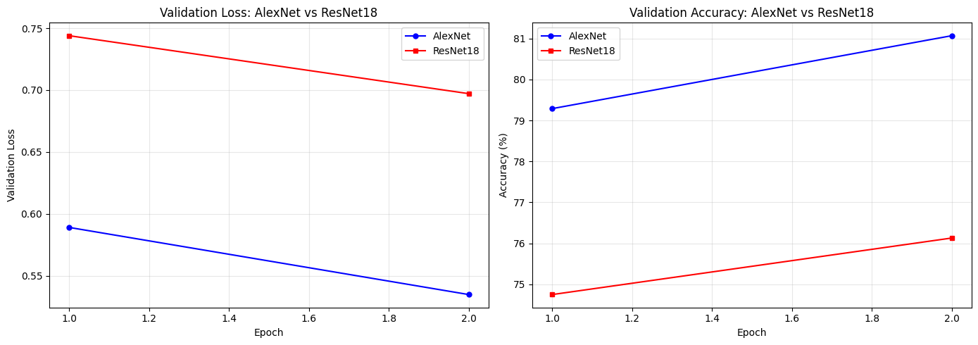
# ── Final comparison table ────────────────────────────────────────────
alexnet_trainable = sum(p.numel() for p in alexnet.parameters() if p.requires_grad)
resnet_trainable  = sum(p.numel() for p in resnet.parameters()  if p.requires_grad)
effnet_trainable  = sum(p.numel() for p in effnet.parameters()  if p.requires_grad)
alexnet_total     = sum(p.numel() for p in alexnet.parameters())
resnet_total      = sum(p.numel() for p in resnet.parameters())
effnet_total      = sum(p.numel() for p in effnet.parameters())

print('=' * 95)
print(f"{'Metric':<35} {'AlexNet':>18} {'ResNet18':>18} {'EfficientNet-B0':>18}")
print('=' * 95)
print(f"{'Total parameters':<35} {alexnet_total:>18,} {resnet_total:>18,} {effnet_total:>18,}")
print(f"{'Trainable parameters':<35} {alexnet_trainable:>18,} {resnet_trainable:>18,} {effnet_trainable:>18,}")
print(f"{'Final val accuracy':<35} {alexnet_history['val_acc'][-1]:>17.2f}% {resnet_history['val_acc'][-1]:>17.2f}% {effnet_history['val_acc'][-1]:>17.2f}%")
print(f"{'Year introduced':<35} {'2012':>18} {'2015':>18} {'2019':>18}")
print(f"{'Head replaced':<35} {'classifier[6]':>18} {'fc':>18} {'classifier[1]':>18}")
print('=' * 95)
===========================================================================
Metric AlexNet ResNet18
===========================================================================
Total parameters 57,044,810 11,181,642
Trainable parameters 40,970 5,130
Final val accuracy 81.07% 76.13%
Year introduced 2012 2015
Head replaced classifier[6] fc
===========================================================================
Key Observations
1. Very few parameters are actually trained.
Both models freeze the backbone and train only the final classifier head.
For ResNet18 that head is especially small (512→10), so transfer learning is very lightweight.
2. Both models converge quickly.
With only a tiny classifier head learning, most of the useful feature extraction is already done by the pretrained backbone.
3. ResNet18 is a more modern design than AlexNet.
Residual connections make deeper networks easier to optimise, and the architecture is far more parameter-efficient than AlexNet.
4. Architecture matters even when the backbone is frozen.
The forward pass still depends on the quality of the pretrained features, so a stronger backbone can produce a better linear-separation problem for the new head.
✅ Check Your Understanding — Final
Q7: You have a dataset of 500 medical X-ray images (chest/no-chest). Should you train from scratch or use transfer learning? Which strategy?
A) Train from scratch — medical images are very different from ImageNet
B) Transfer learning — freeze the backbone and train only a new classifier head, because 500 images is too small to train a deep network from scratch
C) Transfer learning — unfreeze all layers and fine-tune everything, because medical images differ a lot from natural images
D) Neither — 500 images is too few for any deep learning approach
Click to reveal solution
Answer: B)
500 images is far too few to learn a CNN from scratch — you’d overfit badly.
Transfer learning works well even for medical images, because early CNN layers (edges, textures) are universal and still useful. With only 500 images, freezing the backbone is safer than fine-tuning all layers (which risks catastrophic forgetting and overfitting).
Q8: What would happen if you forgot to apply ImageNet normalisation when using a pretrained model?
A) Nothing — the model will learn to compensate
B) The model would predict random classes
C) The activations in the early layers would be far outside the range the model was optimised for, degrading the pretrained features and likely resulting in poor accuracy
D) A PyTorch error would be raised
Click to reveal solution
Answer: C)
The pretrained weights encode patterns relative to inputs with ImageNet statistics.
Without normalisation, the first-layer activations will be very different from what those weights expect, and the useful features won’t fire correctly. In practice, you’ll see noticeably lower accuracy, but no PyTorch error — the model still runs, it just performs poorly.
Part 9 — Visualising What the Models Learned (~10 min)
A great sanity check is to look at which images each model gets wrong — and whether both models fail on the same examples. Shared failures often reveal something about the data, not the model.
What to look for
In the error grids (next two cells):
Do both models fail on the same images? If yes, those images are probably just hard — blurry, unusual angle, or ambiguous even to a human eye.
Does one model fail where the other succeeds? That reveals a difference in the features each backbone learned.
Which classes appear most often in the wrong predictions? E.g., cats/dogs are often confused because both are furry animals photographed in similar settings.
In the per-class bar chart:
Which classes have high accuracy (>70%)? These likely have very distinctive visual features (e.g., airplane silhouettes are unique).
Which classes are low (<50%)? These likely look similar to another class from CIFAR-10’s angle (e.g., cats vs. dogs, automobiles vs. trucks).
Does ResNet18 do better on every class, or only some? That tells you where the stronger backbone features make a difference.
Comparing Model Mistakes
Looking at misclassified test images is a useful sanity check. The two plots below show the first 16 mistakes for AlexNet and ResNet18.
Each image title shows True class → Predicted class in red.
Look for patterns: are the mistakes reasonable (the wrong class looks similar)?
Or are they totally random?
Example of a reasonable mistake: A truck image misclassified as “automobile” — both have four wheels, metal body, similar colours in small 32×32 images.
Example of an unreasonable mistake: A ship misclassified as “cat” — this suggests the model is not generalising well and may need more training or fine-tuning.
Source
def collect_errors(model, loader, device, max_errors=16):
    """Return (images, true_labels, pred_labels) for the first max_errors mistakes."""
    model.eval()
    wrong_imgs, wrong_true, wrong_pred = [], [], []
    with torch.no_grad():
        for images, labels in loader:
            outputs = model(images.to(device))
            _, preds = outputs.max(1)
            preds = preds.cpu()
            mask  = preds != labels          # True where the model is wrong
            wrong_imgs.extend(images[mask])
            wrong_true.extend(labels[mask])
            wrong_pred.extend(preds[mask])
            if len(wrong_imgs) >= max_errors:
                break
    return wrong_imgs[:max_errors], wrong_true[:max_errors], wrong_pred[:max_errors]


alex_errs, alex_true, alex_pred = collect_errors(alexnet, test_loader, device)
resnet_errs, resnet_true, resnet_pred = collect_errors(resnet, test_loader, device)
effnet_errs, effnet_true, effnet_pred = collect_errors(effnet, test_loader, device)

fig, axes = plt.subplots(2, 8, figsize=(18, 5))
fig.suptitle('AlexNet — First 16 Misclassified Test Images', fontsize=12)
for i, ax in enumerate(axes.ravel()):
    if i < len(alex_errs):
        img = denormalize(alex_errs[i])
        ax.imshow(img.permute(1, 2, 0).numpy())
        ax.set_title(f'T:{CLASS_NAMES[alex_true[i]]}\nP:{CLASS_NAMES[alex_pred[i]]}',
                     fontsize=7, color='red')
    ax.axis('off')
plt.tight_layout()
plt.show()

fig, axes = plt.subplots(2, 8, figsize=(18, 5))
fig.suptitle('ResNet18 — First 16 Misclassified Test Images', fontsize=12)
for i, ax in enumerate(axes.ravel()):
    if i < len(resnet_errs):
        img = denormalize(resnet_errs[i])
        ax.imshow(img.permute(1, 2, 0).numpy())
        ax.set_title(f'T:{CLASS_NAMES[resnet_true[i]]}\nP:{CLASS_NAMES[resnet_pred[i]]}',
                     fontsize=7, color='red')
    ax.axis('off')
plt.tight_layout()
plt.show()

fig, axes = plt.subplots(2, 8, figsize=(18, 5))
fig.suptitle('EfficientNet-B0 — First 16 Misclassified Test Images', fontsize=12)
for i, ax in enumerate(axes.ravel()):
    if i < len(effnet_errs):
        img = denormalize(effnet_errs[i])
        ax.imshow(img.permute(1, 2, 0).numpy())
        ax.set_title(f'T:{CLASS_NAMES[effnet_true[i]]}\nP:{CLASS_NAMES[effnet_pred[i]]}',
                     fontsize=7, color='red')
    ax.axis('off')
plt.tight_layout()
plt.show()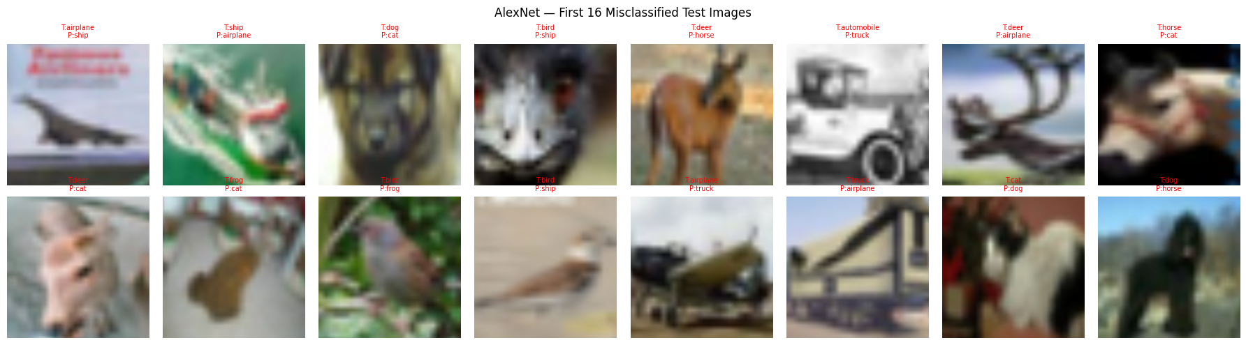
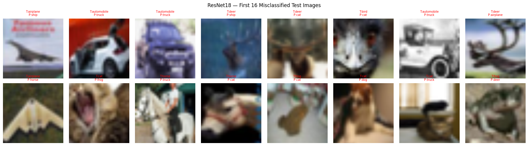
Confusion Matrix
A confusion matrix shows which classes get confused for which other classes. Each row = the true class; each column = what the model predicted. A perfect model would have dark blue only on the diagonal and light (near-zero) everywhere else.
How to read it:
Dark diagonal → the model is correct for that class
Off-diagonal bright squares → the model confuses those two classes
Compare AlexNet and ResNet18 rows: if one model has a brighter off-diagonal square, it makes that mistake more often
Common confusions to watch for in CIFAR-10:
cat↔dog(similar textures at 32×32)automobile↔truck(similar shapes)deer↔horseorbird(similar body shapes)
Source
# ── Confusion matrices for AlexNet, ResNet18 and EfficientNet-B0 ─────────────────────────────
def compute_confusion_matrix(model, loader, device, n_classes=10):
    """Return an n×n confusion matrix (counts)."""
    cm = np.zeros((n_classes, n_classes), dtype=int)
    model.eval()
    with torch.no_grad():
        for images, labels in loader:
            outputs = model(images.to(device))
            _, preds = outputs.max(1)
            preds  = preds.cpu().numpy()
            labels = labels.numpy()
            for t, p in zip(labels, preds):
                cm[t][p] += 1
    return cm

cm_alex   = compute_confusion_matrix(alexnet, test_loader, device)
cm_resnet = compute_confusion_matrix(resnet,  test_loader, device)
cm_effnet = compute_confusion_matrix(effnet,  test_loader, device)

fig, axes = plt.subplots(1, 3, figsize=(20, 6))

models_cm = [
    (cm_alex,   'AlexNet'),
    (cm_resnet, 'ResNet18'),
    (cm_effnet, 'EfficientNet-B0')
]

for ax, (cm, title) in zip(axes, models_cm):
    cm_norm = cm.astype(float) / cm.sum(axis=1, keepdims=True)   # normalise by row
    im = ax.imshow(cm_norm, cmap='Blues', vmin=0, vmax=1)
    ax.set_xticks(range(10));  ax.set_yticks(range(10))
    ax.set_xticklabels(CLASS_NAMES, rotation=45, ha='right', fontsize=9)
    ax.set_yticklabels(CLASS_NAMES, fontsize=9)
    ax.set_xlabel('Predicted class', fontsize=10)
    ax.set_ylabel('True class', fontsize=10)
    ax.set_title(f'{title} — Confusion Matrix', fontsize=11)
    # Annotate cells with values
    for i in range(10):
        for j in range(10):
            ax.text(j, i, f'{cm_norm[i, j]:.2f}',
                    ha='center', va='center',
                    fontsize=7,
                    color='white' if cm_norm[i, j] > 0.5 else 'black')

plt.suptitle('Normalised Confusion Matrices — diagonal = correct, off-diagonal = errors', fontsize=12)
plt.tight_layout()
plt.show()
Per-Class Accuracy
Overall accuracy can hide which CIFAR-10 classes are easy or difficult. This section breaks accuracy down by class and prints a table for side-by-side comparison for AlexNet and ResNet18.
How to read the bar chart:
A tall bar = the model is good at that class
A short bar = the model struggles — often because that class looks similar to another
Typical easy classes: airplane, ship (distinctive shapes)
Typical hard classes: cat, dog (similar textures and shapes at 32×32 resolution)
Discussion question: If AlexNet gets 40% on “cat” but ResNet18 gets 60%, what does that suggest about the quality of features each backbone learned?
def per_class_accuracy(model, loader, device, n_classes=10):
    """Return accuracy per class as a list."""
    model.eval()
    correct = [0] * n_classes
    total   = [0] * n_classes
    with torch.no_grad():
        for images, labels in loader:
            outputs = model(images.to(device))
            _, preds = outputs.max(1)
            preds = preds.cpu()
            for c in range(n_classes):
                mask       = labels == c
                correct[c] += preds[mask].eq(labels[mask]).sum().item()
                total[c]   += mask.sum().item()
    return [100.0 * correct[c] / total[c] if total[c] > 0 else 0.0 for c in range(n_classes)]


alex_class_acc = per_class_accuracy(alexnet, test_loader, device)
resnet_class_acc = per_class_accuracy(resnet, test_loader, device)
effnet_class_acc = per_class_accuracy(effnet, test_loader, device)

x = np.arange(len(CLASS_NAMES))
width = 0.25
fig, ax = plt.subplots(figsize=(14, 6))
ax.bar(x - width, alex_class_acc, width, label='AlexNet',  color='steelblue')
ax.bar(x,         resnet_class_acc,  width, label='ResNet18',    color='tomato')
ax.bar(x + width, effnet_class_acc,  width, label='EfficientNet-B0', color='forestgreen')

ax.set_xticks(x)
ax.set_xticklabels(CLASS_NAMES, rotation=20, ha='right')
ax.set_ylabel('Accuracy (%)')
ax.set_title('Per-class Accuracy Comparison')
ax.legend()
ax.set_ylim(0, 100)
ax.axhline(y=10, color='gray', linestyle='--', alpha=0.5, label='Random (10%)')
ax.grid(True, alpha=0.3, axis='y')
plt.tight_layout()
plt.show()

print(f"{'Class':<15} {'AlexNet':>8} {'ResNet18':>8} {'EffNet-B0':>8}")
print('-' * 45)
for cls, a, r, e in zip(CLASS_NAMES, alex_class_acc, resnet_class_acc, effnet_class_acc):
    print(f"{cls:<15} {a:>7.1f}% {r:>7.1f}% {e:>7.1f}%")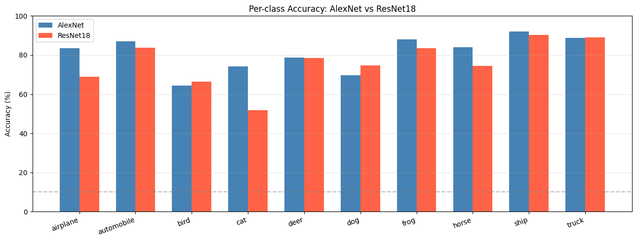
Class            AlexNet ResNet18
-----------------------------------
airplane           83.6%    69.0%
automobile         87.1%    83.8%
bird               64.3%    66.4%
cat                74.3%    51.8%
deer               78.7%    78.4%
dog                69.8%    74.6%
frog               88.1%    83.4%
horse              84.0%    74.5%
ship               92.0%    90.4%
truck              88.8%    89.0%
Summary
The Transfer Learning Recipe (5 Steps)
Every transfer learning task follows the same pattern. Memorise this:
Step 1 — Load pretrained model
         model = models.resnet18(weights=ResNet18_Weights.DEFAULT)

Step 2 — Freeze all backbone parameters
         for param in model.parameters():
             param.requires_grad = False

Step 3 — Replace the final layer for your task
         model.fc = nn.Linear(model.fc.in_features, NUM_CLASSES)

Step 4 — Move model to device
         model = model.to(device)

Step 5 — Train only the new head
         optimizer = optim.Adam(
             filter(lambda p: p.requires_grad, model.parameters()), lr=1e-3
         )
This exact 5-step recipe works for AlexNet, ResNet18, VGG, EfficientNet, and most other torchvision models. Only Step 3 changes (the layer name differs per model).
What We Covered
| Concept | Key Takeaway |
|---|---|
| ImageNet | 1.2M images, 1000 classes — the dataset used to pre-train these models |
| Transfer learning | Reuse features learned on large datasets; only train a new classifier head |
| Freezing parameters | requires_grad = False prevents weights from being updated; saves memory and compute |
| ImageNet normalisation | Pre-trained models expect inputs normalised with ImageNet statistics |
| 224×224 resizing | AlexNet and ResNet18 were designed for ImageNet-sized inputs |
| AlexNet classifier[6] | The final Linear(4096→1000) layer; we replace it with Linear(4096→10) |
ResNet fc layer | The final Linear(512→1000) layer; we replace it with Linear(512→10) |
| EfficientNet classifier[1] | The final Linear(1280→1000) layer; we replace it with Linear(1280→10) |
| Residual connection | Adds the input back to the block output, helping optimisation and gradient flow |
| Cosine LR schedule | Smoothly reduces LR from initial value to near 0 for stable convergence |
When to Use Transfer Learning
| Situation | Recommended Strategy |
|---|---|
| Small dataset (<10K images) | Freeze all backbone layers, train only the head |
| Medium dataset (10K–100K) | Freeze early layers; fine-tune later layers + head |
| Large dataset (>100K) | Fine-tune the entire network from the pretrained weights |
| Very different domain (e.g., satellite images, medical scans) | Consider fine-tuning more layers, or use domain-specific pretrained models |
What’s Next?
In the next tutorial we can build on this by exploring deeper fine-tuning, learning-rate strategies, or more efficient modern backbones such as EfficientNet.