In this tutorial, we will build an understanding of how modern large language models (LLMs) like ChatGPT, Claude, and Gemini work under the hood. The key innovation behind all of these models is the Transformer architecture, introduced in the landmark 2017 paper “Attention Is All You Need” by Vaswani et al.
We will walk through every major component step by step, with analogies and diagrams so you can see exactly how each piece works. No prior knowledge of Transformers is assumed — we will build everything from the ground up.
Learning Outcomes
By the end of this tutorial, you will be able to:
Explain what a language model is and why predicting the next word is so powerful.
Describe how raw text becomes numbers through tokenization and vocabulary lookup.
Explain what word embeddings are and why they capture meaning as vectors.
Understand positional encoding and why Transformers need it (unlike RNNs).
Articulate the limitations of RNNs and why self-attention was invented.
Walk through the self-attention mechanism step by step, including Query, Key, and Value.
Explain multi-head attention and why multiple “perspectives” help.
Describe masked (causal) attention and why it is essential for text generation.
Understand the full Transformer block including residual connections, layer normalization, and feed-forward layers.
Use a pretrained Transformer model through the Hugging Face library.
Prerequisites
Basic understanding of neural networks (from Tutorials 1-4)
Familiarity with RNNs (from Tutorial 8)
Part 1 — What Is a Language Model?
Before we dive into Transformers, we need to understand the fundamental task they are trained to do: language modeling.
The Core Idea
A language model is a system that estimates the probability of text sequences. The most common formulation is next-token prediction: given a sequence of words (or tokens), what word is most likely to come next?
For example, consider the sentence prefix:
“Money can’t buy ___”
A good language model should assign:
High probability to words like “happiness”, “love”, “time” — these are plausible continuations
Low probability to words like “refrigerator”, “purple”, “running” — these don’t fit the context
Mathematically, we write this as:
This reads: “the probability of the next word, given all the words that came before it.”
Why Is This So Powerful?
You might think: “Predicting the next word? That sounds too simple to be useful.” But here is the key insight — a model that is truly excellent at predicting the next word must understand language deeply. To predict well, the model must learn:
Grammar and syntax — it needs to know what word types can follow others
Semantics and meaning — it needs to understand what the sentence is about
World knowledge — it needs facts about the world to make good predictions
Reasoning — it sometimes needs to follow logical chains
This is why the same next-token prediction objective can power such diverse applications:
| Application | How language modeling helps |
|---|---|
| Autocomplete | Directly predict the next word as you type |
| Chatbots (ChatGPT, Claude) | Generate responses one token at a time |
| Translation | Given source text, predict target language tokens |
| Summarization | Given a document, predict a shorter version |
| Code generation | Given a description, predict code tokens |
| Speech recognition | Choose the most probable text from ambiguous audio |
Part 1 — Check Your Understanding
Question 1.1: What is the core task of a language model?
A) Translating text from one language to another
B) Estimating the probability of the next token given the previous tokens
C) Converting speech to text
D) Classifying documents into categories
YOUR ANSWER HERE
Question 1.2: Why does a model that is excellent at next-word prediction need to understand more than just grammar?
A) Because grammar rules are too complex for neural networks
B) Because predicting contextually plausible words often requires world knowledge, semantics, and reasoning — not just knowing which word types can follow others
C) Because next-word prediction only works on English text
D) Because grammar is not related to language modeling
YOUR ANSWER HERE
Question 1.3: Which of the following applications is not directly powered by language modeling?
A) Autocomplete suggestions on your phone
B) ChatGPT generating a response to your question
C) Adjusting the brightness of your laptop screen
D) Code generation from a natural language description
YOUR ANSWER HERE
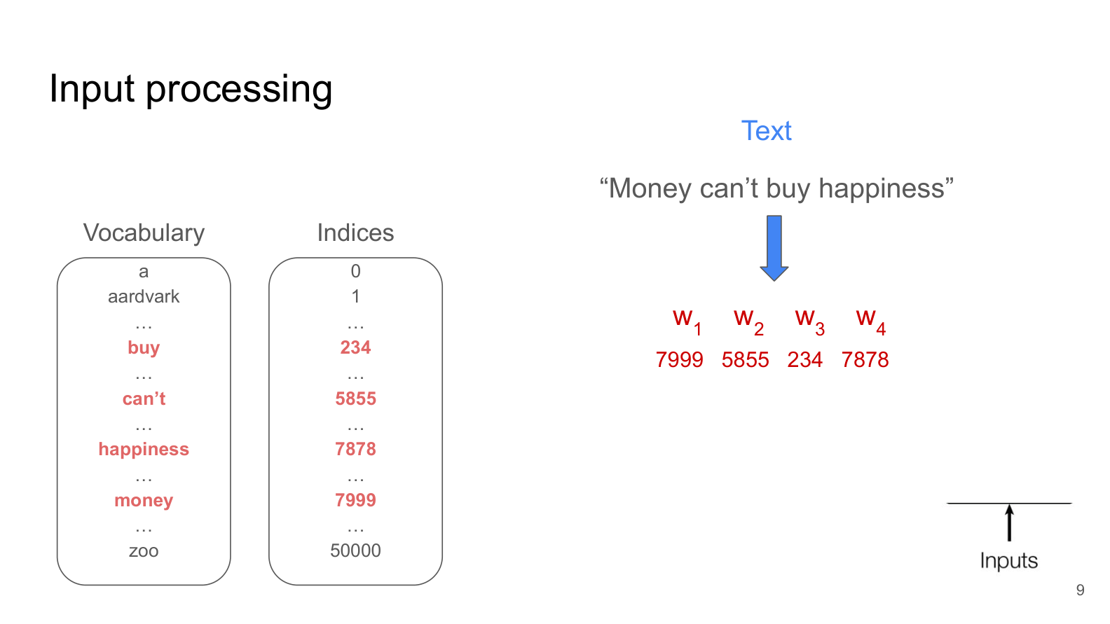
Part 2 — From Text to Numbers: Tokenization and Input Processing
Neural networks cannot work with raw text directly — they only understand numbers. So before any learning can happen, we need to convert text into numerical form. This happens in two stages: tokenization and vocabulary lookup.
Step 1: Tokenization — Breaking Text into Pieces
Tokenization is the process of splitting text into smaller units called tokens. A token might be:
A whole word:
"money","happiness"A subword:
"un"+"happi"+"ness"(this is what modern models like GPT and BERT actually use)A single character:
"m","o","n","e","y"
Modern LLMs typically use subword tokenization (like Byte-Pair Encoding or WordPiece). This is a middle ground: common words stay whole, but rare words get split into recognizable pieces. For example, the word “unhappiness” might become ["un", "happi", "ness"].
Step 2: Vocabulary Lookup — Mapping Tokens to Numbers
Every model has a fixed vocabulary — a dictionary that maps each known token to a unique integer (called an index or token ID).
As shown in the slide above:
The word
"money"might map to index 7999The word
"can't"might map to index 5855The word
"buy"might map to index 234The word
"happiness"might map to index 7878
So the sentence “Money can’t buy happiness” becomes a sequence of integers: [7999, 5855, 234, 7878].
Think of it like a phone book: each word has a unique “phone number” (its index), and the model uses these numbers to look up information about each word.
Part 2 — Check Your Understanding
Question 2.1: What is the purpose of tokenization?
A) To translate words into a different language
B) To split text into smaller units (tokens) that can be mapped to numerical IDs
C) To remove punctuation from text
D) To check if the text is grammatically correct
YOUR ANSWER HERE
Question 2.2: In subword tokenization, the word “unhappiness” might be split into ["un", "happi", "ness"]. Why is this approach preferred over whole-word tokenization?
A) It makes the vocabulary smaller while still being able to represent any word — even rare or unseen words — by combining known subword pieces
B) It makes the text shorter
C) It is faster to compute than whole-word tokenization
D) It removes the need for a vocabulary entirely
YOUR ANSWER HERE
Question 2.3: If a vocabulary maps “buy” to index 234 and “sell” to index 9012, what can we say about the relationship between these two words based on their indices alone?
A) They are antonyms because their indices are far apart
B) Nothing — token indices are arbitrary labels with no semantic meaning
C) “buy” is more common because it has a lower index
D) They are related because they are both verbs
YOUR ANSWER HERE
Part 3 — Word Embeddings: Giving Meaning to Numbers
We now have token IDs (integers), but a raw integer like 234 doesn’t tell the model anything about what the word means. The number 234 for “buy” and 235 for some other word have no meaningful relationship — they’re just arbitrary labels.
Embeddings solve this problem by mapping each token ID to a dense vector (a list of numbers) that captures the token’s meaning.
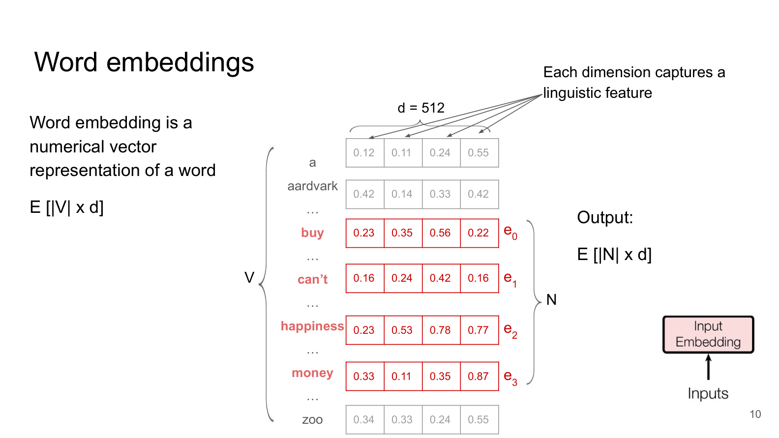
How Embeddings Work
An embedding layer is essentially a large lookup table (matrix) with:
Rows = one for each token in the vocabulary (e.g., 50,000 rows)
Columns = the embedding dimension
d(e.g., 512 numbers per token)
When the model sees token ID 234 (the word “buy”), it simply looks up row 234 in this table and retrieves a vector of d numbers, like [0.23, 0.35, 0.56, 0.22, ...].
The Analogy: GPS Coordinates for Words
Think of embeddings as GPS coordinates in a “meaning space”:
Words with similar meanings end up at nearby coordinates
“king” and “queen” are close together
“cat” and “kitten” are close together
Words with different meanings are far apart
“king” and “banana” are far apart
The beautiful thing is that these coordinates are learned during training — the model figures out where to place each word in this space by reading billions of sentences. Nobody manually assigns these vectors.
Key Properties of Learned Embeddings
Semantic similarity: Words used in similar contexts get similar vectors
Analogies emerge: The famous example:
king - man + woman ≈ queenEach dimension captures something: One dimension might relate to “animate vs. inanimate”, another to “positive vs. negative sentiment”, etc. (though in practice, dimensions are not so neatly interpretable)
The Math
If our vocabulary has |V| tokens and we choose embedding dimension d, the embedding matrix E has shape |V| × d.
For an input sequence of N tokens, the embedding layer outputs a matrix of shape N × d — one d-dimensional vector per token.
Part 3 — Check Your Understanding
Question 3.1: What is a word embedding?
A) A one-hot encoded vector where only one element is 1
B) A dense vector of learned numbers that captures the semantic meaning of a token
C) The position of a word in the vocabulary
D) A binary representation of the word’s characters
YOUR ANSWER HERE
Question 3.2: If two words consistently appear in similar contexts across billions of sentences (e.g., “dog” and “cat” both appear in “The ___ sat on the mat”), what would you expect about their embedding vectors?
A) They would be identical vectors
B) They would be close together in embedding space because they are used in similar contexts
C) They would be far apart because they are different words
D) They would have the same token ID
YOUR ANSWER HERE
Question 3.3: The embedding matrix for a model with a vocabulary of 50,000 tokens and an embedding dimension of 512 has shape 50,000 x 512. How many learnable parameters does this single layer contain?
A) 50,000
B) 512
C) 25,600,000 (50,000 x 512)
D) 50,512
YOUR ANSWER HERE
Part 4 — Positional Encoding: Teaching the Model About Word Order
We have one more problem to solve before we can build a Transformer. Consider these two sentences:
“The cat chased the mouse”
“The mouse chased the cat”
These sentences have completely different meanings, but they contain the exact same words! If we only use embeddings, both sentences would produce the same set of vectors (just in a different order) — and the Transformer’s attention mechanism (which we’ll learn next) processes all tokens simultaneously rather than one at a time. So it wouldn’t even know the order.
Positional encoding solves this by injecting information about each token’s position in the sequence.
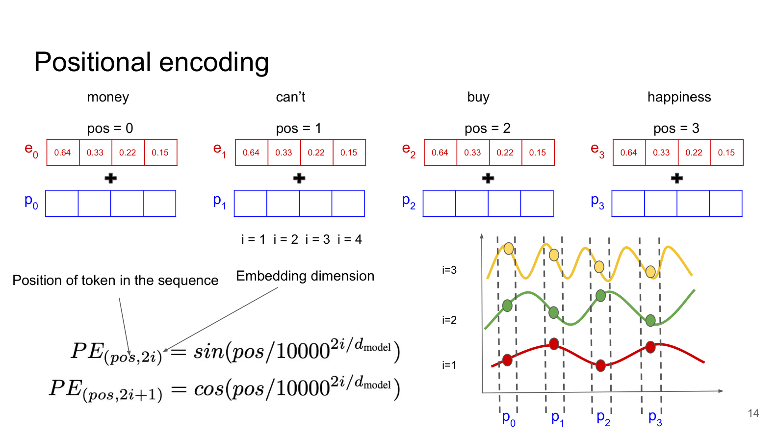
How Positional Encoding Works
The original Transformer uses sinusoidal positional encoding. The idea is:
For each position in the sequence (position 0, 1, 2, ...), generate a unique vector of the same size as the embedding (
ddimensions).Add this position vector to the token’s embedding vector.
The result: each token’s representation now contains both its meaning (from the embedding) AND its position (from the positional encoding).
Why Sinusoidal Functions?
The positional encoding uses sine and cosine waves at different frequencies:
Where:
pos= the position of the token in the sequence (0, 1, 2, ...)i= the dimension index (which of thednumbers we’re computing)d_model= the total embedding dimension
Why this specific formula? Three key reasons:
Each position gets a unique pattern: No two positions produce the same vector
Relative positions are easy to learn: The model can learn to attend to “the word 3 positions ago” because the mathematical relationship between position vectors is consistent
Generalizes to unseen lengths: Unlike learned position embeddings, sinusoidal encodings work for sequences longer than any seen during training
The Analogy: A Clock
Think of positional encoding like reading a clock. The hour hand moves slowly (low frequency), the minute hand moves faster (medium frequency), and the second hand moves fastest (high frequency). By looking at all three hands together, you know exactly what time it is. Similarly, by combining sine waves at different frequencies across dimensions, each position gets a unique “timestamp.”
Part 4 — Check Your Understanding
Question 4.1: Why do Transformers need positional encoding, while RNNs do not?
A) Because Transformers have more parameters than RNNs
B) Because RNNs process tokens sequentially (so order is implicit), while Transformers process all tokens simultaneously and would otherwise have no information about word order
C) Because positional encoding makes the model faster
D) Because RNNs cannot handle long sequences
YOUR ANSWER HERE
Question 4.2: How is positional encoding combined with the token embedding?
A) The positional encoding replaces the token embedding
B) The positional encoding is concatenated (appended) to the token embedding, doubling its size
C) The positional encoding is added (element-wise) to the token embedding, keeping the same size
D) The positional encoding is multiplied with the token embedding
YOUR ANSWER HERE
Question 4.3: Consider the sentences “The cat chased the mouse” and “The mouse chased the cat.” Without positional encoding, how would a Transformer treat these two sentences?
A) It would understand them perfectly because the embeddings are different
B) It would treat them as having the same meaning because the same set of token embeddings would be produced (just in a different order), and without positional encoding the model has no way to distinguish the order
C) It would crash because the sentences have different meanings
D) It would always prefer the first sentence
YOUR ANSWER HERE
Part 5 — From RNNs to Self-Attention: Why We Needed a New Approach
In Tutorial 8, we learned about Recurrent Neural Networks (RNNs) and LSTMs. These models process sequences one token at a time, passing information forward through a hidden state. While this works, it has three major problems that become critical when processing long sequences:
Problem 1: Sequential Processing (Slow)
RNNs process tokens one at a time, in order. To process the 100th word, you must first process words 1 through 99. This means:
Training cannot be parallelized across time steps
On modern GPUs (which excel at parallel computation), this is extremely wasteful
Training on large datasets takes a very long time
Problem 2: The Bottleneck (Forgetting)
All information from the past must squeeze through a single fixed-size hidden state vector. Imagine trying to summarize an entire book into a single Post-it note, and then reading the next chapter using only that Post-it note as context. Important details inevitably get lost.
Even LSTMs, which were designed to address this with gates and cell states, still struggle with very long sequences (hundreds or thousands of tokens).
Problem 3: Vanishing/Exploding Gradients
During backpropagation through many time steps, gradients can either:
Vanish (shrink to near zero) — the model can’t learn long-range dependencies
Explode (grow extremely large) — training becomes unstable
The Solution: Self-Attention
The Transformer’s self-attention mechanism addresses all three problems:
| Problem | RNN | Self-Attention |
|---|---|---|
| Processing | Sequential (one token at a time) | Parallel (all tokens at once) |
| Long-range dependencies | Information compressed through bottleneck | Direct connection between any two tokens |
| Gradient flow | Through many sequential steps | Direct path in single step |
The key insight: every token can directly “look at” every other token in the sequence, regardless of distance. A word at position 1 can directly interact with a word at position 100, without information having to pass through 99 intermediate steps.
Part 5 — Check Your Understanding
Question 5.1: What is the main problem with the RNN “bottleneck”?
A) RNNs are too fast and skip important information
B) All information about the past must be compressed into a single fixed-size hidden state vector, causing important details to be lost over long sequences
C) RNNs can only process numerical data, not text
D) The bottleneck makes RNNs use too much memory
YOUR ANSWER HERE
Question 5.2: How does self-attention handle long-range dependencies differently from an RNN?
A) Self-attention uses a larger hidden state
B) Self-attention allows any token to directly attend to any other token in a single step, regardless of distance, rather than passing information through many sequential steps
C) Self-attention processes tokens one at a time, but faster
D) Self-attention ignores distant tokens and only looks at nearby ones
YOUR ANSWER HERE
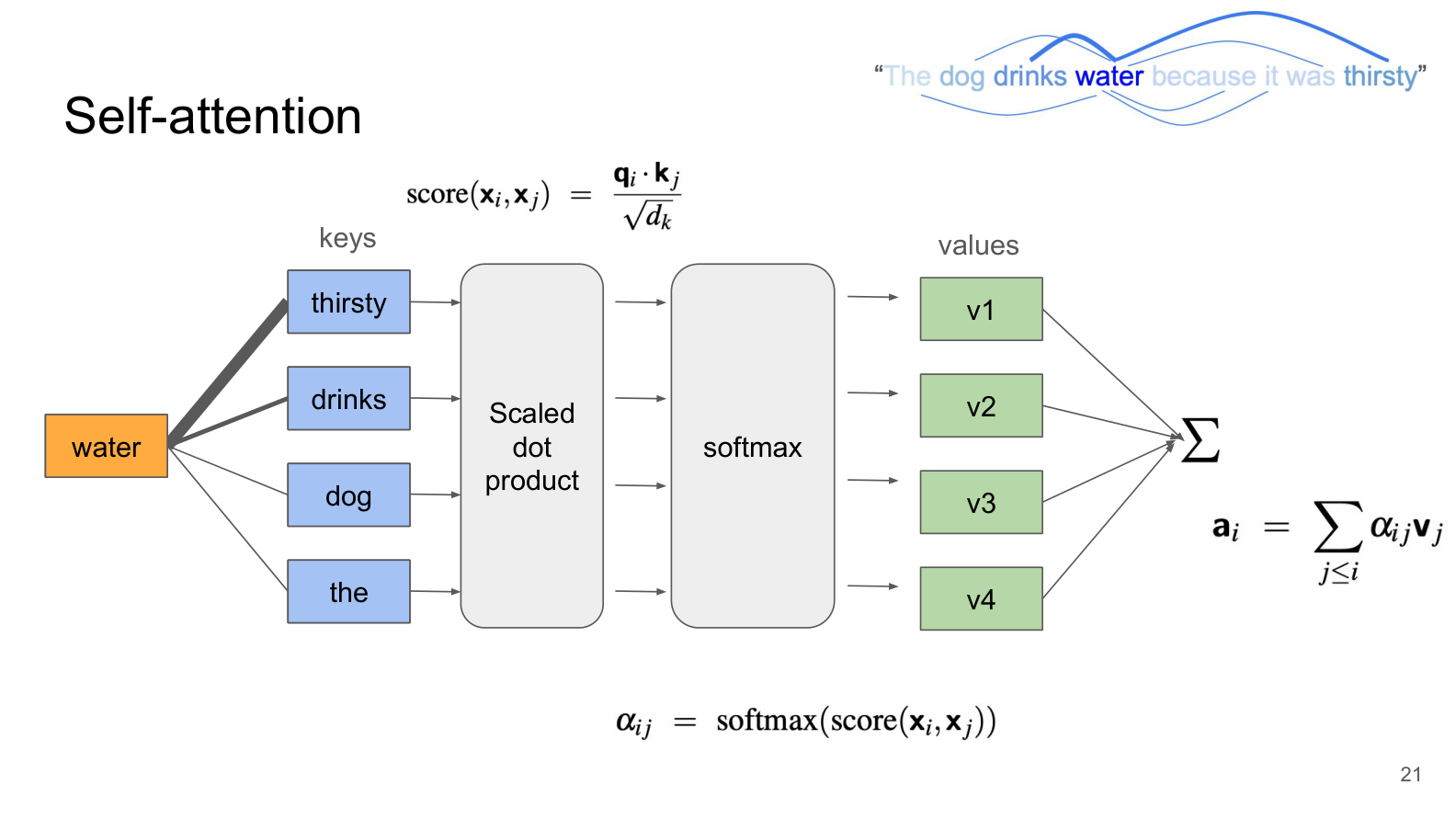
Part 6 — Self-Attention: The Heart of the Transformer
Self-attention is the core mechanism that makes Transformers work. Let’s build it up step by step.
The Intuition: A Classroom Discussion
Imagine a classroom where every student (token) wants to understand the full context of a discussion. Each student:
Has a question they want answered (their Query)
Advertises what they know about (their Key)
Has actual information to share (their Value)
The process:
Each student looks at everyone else’s “Key” (advertisement) and compares it to their own “Query” (question)
If a Key matches a Query well, the student pays more attention to that person
The student then collects information (Values) from everyone, weighted by how relevant each person is
This is exactly how self-attention works!
The Formal Mechanism: Query, Key, Value
Given input embeddings (with positional encoding added), self-attention works in 5 steps:
Step 1: Create Q, K, V vectors
Each token’s embedding is transformed into three different vectors using three separate learned weight matrices:
Where X is the input matrix (shape: N × d_model) and W_Q, W_K, W_V are learned weight matrices (shape: d_model × d_k).
Query (Q): “What am I looking for?” — represents what this token wants to know
Key (K): “What do I have to offer?” — represents what this token can tell others
Value (V): “Here is my actual information” — the content that gets passed along
Step 2: Compute attention scores
For each pair of tokens, compute how relevant they are to each other using the dot product of the Query and Key:
A high dot product means the Query and Key are “pointing in the same direction” — they’re a good match.
Step 3: Scale the scores
Divide by (the square root of the key dimension):
Why scale? Without scaling, when d_k is large, the dot products can become very large numbers. When we then apply softmax, these large values push the output toward one-hot vectors (all attention on one token, none on others). Scaling keeps the values in a range where softmax produces a smoother, more useful distribution.
Step 4: Apply softmax to get attention weights
Softmax converts the raw scores into probabilities that sum to 1. Now each token has a distribution over all other tokens saying “how much should I attend to each?”
Step 5: Compute the weighted sum of Values
Each token’s output is a weighted blend of all tokens’ Value vectors, where the weights come from the attention scores. Tokens that are more “relevant” contribute more to the output.
The Complete Formula
This single formula captures all 5 steps!
A Concrete Example: Why Self-Attention Matters
Consider the sentence from the slide: “The dog drinks water because it was thirsty”
When processing the word “it”, the model needs to figure out: what does “it” refer to? Is it the dog? The water?
With self-attention, the model can directly compare “it” (as a Query) against every other word (as Keys). Through training, it learns that:
“it” should attend strongly to “dog” (because “dog” is the thing that is thirsty)
“it” should attend less to “water” or “the”
This is exactly what the slide shows — the word “water” attends most strongly to “drinks” and “thirsty” because those words are most relevant to understanding “water” in this context.
Part 6 — Check Your Understanding
Question 6.1: In self-attention, what do the Query (Q), Key (K), and Value (V) represent?
A) Q is the input text, K is the output text, V is the translation
B) Q represents what a token is looking for, K represents what a token advertises about itself, and V carries the actual information to be passed along
C) Q, K, and V are three copies of the same vector
D) Q is for questions, K is for keywords, V is for vocabulary
YOUR ANSWER HERE
Question 6.2: Why are the attention scores divided by (the square root of the key dimension) before applying softmax?
A) To make the computation faster
B) Because without scaling, large dot products push softmax toward extreme values (nearly one-hot), producing less useful attention distributions
C) To ensure the output vectors have unit length
D) To reduce the number of parameters
YOUR ANSWER HERE
Question 6.3: In the sentence “The bank by the river was flooded”, which word(s) should “bank” attend to most strongly to correctly interpret its meaning?
A) “The” and “was” — because they are grammatically connected
B) “river” and “flooded” — because they disambiguate that “bank” refers to a riverbank, not a financial institution
C) “by” and “the” — because they are the closest words
D) Only itself — each token should primarily attend to itself
YOUR ANSWER HERE
Part 7 — Multi-Head Attention: Multiple Perspectives at Once
A single self-attention mechanism learns one way to relate tokens to each other. But language is complex — words relate to each other in many different ways simultaneously:
Syntactic (grammatical): the subject relates to its verb
Semantic (meaning): “dog” relates to “thirsty” (both about the animal’s state)
Positional/Local: adjacent words often relate to each other
Coreference: “it” relates to “dog” (they refer to the same thing)
Trying to capture all of these relationships in a single attention pattern is like trying to take one photograph that simultaneously shows a landscape from the front, side, and top. You need multiple viewpoints.
Multi-head attention solves this by running multiple attention mechanisms (“heads”) in parallel, each free to learn a different type of relationship.
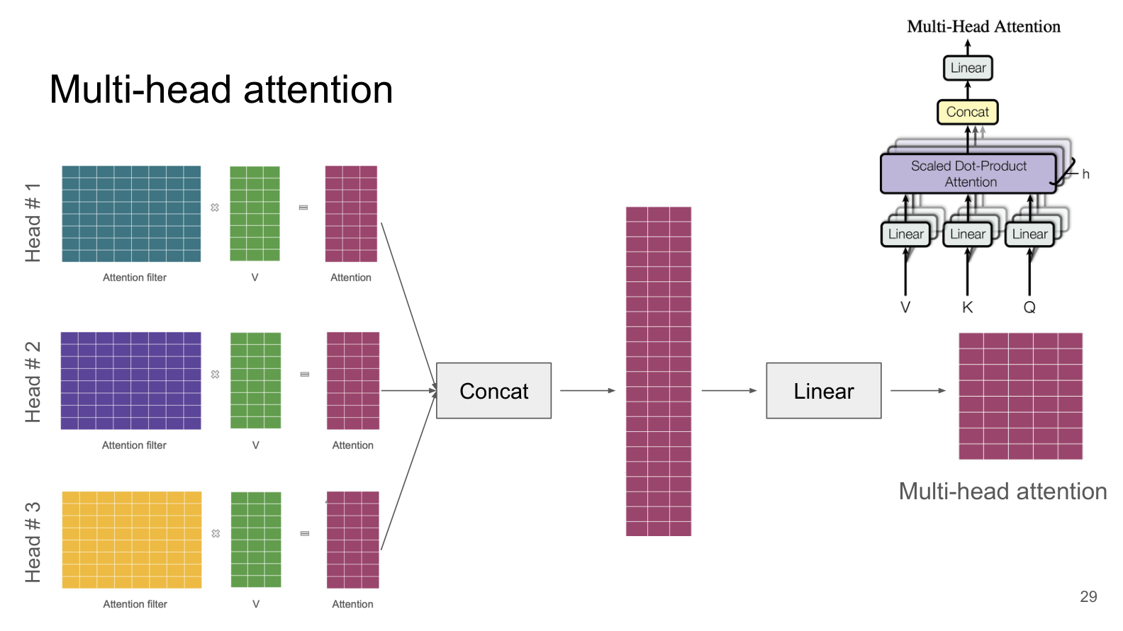
How Multi-Head Attention Works
Split the model dimension into
hheads. Ifd_model = 512andh = 8heads, each head works withd_k = 512 / 8 = 64dimensions.Each head independently computes its own Q, K, V projections and runs self-attention. Each head has its own learned weight matrices, so it can learn to attend to different things.
Concatenate all heads’ outputs back together (back to
d_modeldimensions).Apply a final linear layer to mix the information from different heads.
where each head is:
The Analogy: A Team of Analysts
Think of multi-head attention like a team of analysts reviewing a document:
Analyst 1 focuses on grammatical structure (who did what to whom?)
Analyst 2 focuses on sentiment (is this positive or negative?)
Analyst 3 focuses on temporal relationships (what happened when?)
Analyst 4 focuses on entity relationships (who is related to whom?)
Each analyst writes up their findings independently, and then the results are combined into a comprehensive report. This is far richer than having a single analyst try to track everything at once.
Why Not Just Use a Bigger Single Head?
You might wonder: why not use one big attention head with more dimensions? The answer is that multiple small heads are more expressive than one large head. Each head can specialize in a different pattern, whereas a single large head must compromise between different types of relationships. Research has shown that different heads in trained models do indeed learn distinct attention patterns.
Part 7 — Check Your Understanding
Question 7.1: Why does multi-head attention use multiple attention heads instead of a single larger one?
A) To reduce the total number of parameters
B) Because each head can specialize in a different type of relationship (e.g., syntactic, semantic, positional), which is more expressive than one head trying to capture everything at once
C) Because a single head cannot compute attention at all
D) To make the model run slower but more accurately
YOUR ANSWER HERE
Question 7.2: In a model with d_model = 512 and 8 attention heads, what is the dimension each head works with?
A) 512
B) 8
C) 64 (512 / 8)
D) 4096 (512 x 8)
YOUR ANSWER HERE
Question 7.3: After all heads compute their attention outputs, what happens next?
A) The outputs are averaged together
B) Only the best head’s output is kept
C) The outputs are concatenated back together and passed through a final linear projection
D) The outputs are added element-wise
YOUR ANSWER HERE
Part 8 — Masked (Causal) Attention: Preventing Cheating During Generation
When we use a Transformer to generate text (like ChatGPT writing a response), it produces tokens one at a time, left to right. At each step, the model should only use information from tokens it has already generated — it should not be able to “peek” at future tokens.
But standard self-attention lets every token attend to every other token, including future ones! During training, the entire sequence is available, so without any restriction, the model could trivially “cheat” by looking ahead at the answer.
Masked attention (also called causal attention) solves this by blocking attention to future positions.
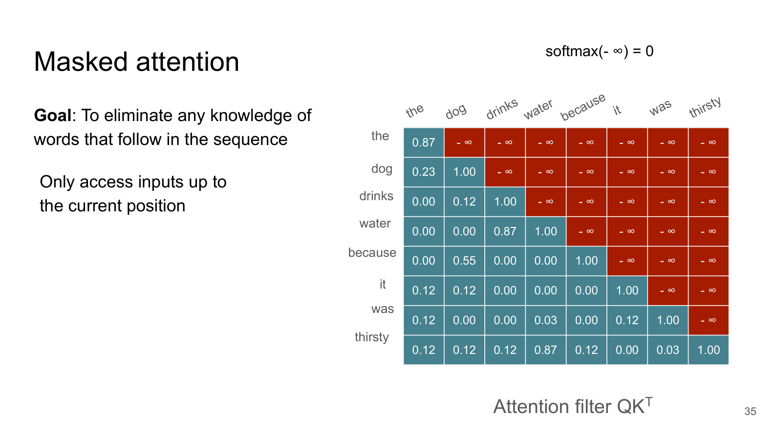
How Masking Works
Look at the slide above. The attention matrix is shown for the sentence “The dog drinks water because it was thirsty”:
Blue cells (lower-left triangle): allowed attention — the token can look at itself and previous tokens
Red cells (upper-right triangle with ): blocked attention — the token cannot look at future tokens
The trick is simple but clever:
Before applying softmax, set all “future” positions to
When softmax encounters , it converts it to 0 (since )
Result: the token effectively “can’t see” future positions
For example, when processing the word “drinks” (position 3):
It can attend to: “the” (pos 1), “dog” (pos 2), “drinks” (pos 3) — itself and past
It cannot attend to: “water” (pos 4), “because” (pos 5), etc. — the future
Why This Is Necessary
Without masking, training and inference would be fundamentally mismatched:
During training: the model sees the complete sentence and could learn to “copy” future tokens instead of truly predicting them
During inference: future tokens don’t exist yet — the model must genuinely predict
Masking ensures that what the model experiences during training exactly matches what it will face during inference. This is critical for the model to learn genuine language understanding rather than shortcut copying.
Part 8 — Check Your Understanding
Question 8.1: Why is causal masking necessary for text generation models like GPT?
A) To make the model run faster during training
B) Because during generation, future tokens don’t exist yet — so the model must learn during training to predict without seeing the future, matching the conditions it will face at inference time
C) To reduce the number of parameters in the model
D) Because the model can only process short sequences
YOUR ANSWER HERE
Question 8.2: In a causal attention mask, which positions are set to before softmax?
A) All positions on the diagonal
B) All positions in the lower-left triangle (past tokens)
C) All positions in the upper-right triangle (future tokens)
D) Random positions selected during each training step
YOUR ANSWER HERE
Question 8.3: What happens when softmax receives a value of ?
A) It outputs 1.0 (maximum attention)
B) It outputs 0.0 (zero attention), effectively blocking that position
C) It crashes with an error
D) It outputs a negative number
YOUR ANSWER HERE
Part 9 — The Full Transformer Block: Putting It All Together
Self-attention is the star of the Transformer, but a complete Transformer block includes several other important components that make training stable and effective. Let’s look at the full picture.
Components of a Transformer Block
Each Transformer block applies these operations in sequence:
Input
  │
  ├──► Multi-Head Attention ──► Add & Layer Norm ──► Feed-Forward Network ──► Add & Layer Norm ──► Output
  │         ▲                        ▲                                              ▲
  └─────────┘ (residual)             │                                              │
                                     └──────────────── (residual) ──────────────────┘
Let’s understand each new component:
1. Residual Connections (Skip Connections)
You already learned about residual connections in CNNs (ResNet). The same idea applies here:
Instead of replacing the input, we add the layer’s output back to the input. This serves two purposes:
Gradient flow: Gradients can flow directly through the skip connection, preventing vanishing gradients in deep networks
Identity fallback: If a layer isn’t helpful, the network can learn to “ignore” it (set its weights near zero) and just pass the input through
2. Layer Normalization
Layer normalization normalizes each token’s representation to have zero mean and unit variance:
Where and are the mean and standard deviation computed across the features (dimensions) for each token independently, and and are learned scale and shift parameters.
Why do we need this? As data flows through many layers, the distribution of values can drift (values might get very large or very small). Layer normalization keeps values in a stable range, which makes training faster and more reliable.
3. Feed-Forward Network (FFN)
After attention, each token’s representation passes through a small two-layer neural network:
This is applied independently to each token (the same network is applied to every position). The inner dimension is typically 4× the model dimension (e.g., d_model=512 → inner dimension = 2048).
Why do we need this? Self-attention is good at mixing information between tokens, but the FFN is where the model does computation within each token. Research suggests that the FFN layers act as a kind of “memory” that stores factual knowledge learned during training.
How a Complete Transformer Model Is Built
A full Transformer model stacks many of these blocks on top of each other:
| Model | Number of Blocks | d_model | Attention Heads |
|---|---|---|---|
| GPT-2 (small) | 12 | 768 | 12 |
| BERT-Base | 12 | 768 | 12 |
| GPT-3 | 96 | 12,288 | 96 |
| LLaMA 2 (70B) | 80 | 8,192 | 64 |
Each block refines the representations. Early blocks might capture basic syntax, middle blocks might capture semantics, and later blocks might capture complex reasoning patterns.
Encoder vs. Decoder: Two Flavors of Transformers
The original 2017 “Attention Is All You Need” paper proposed an encoder-decoder architecture for machine translation. Since then, the community has found that using just one half is often more effective:
| Architecture | Attention Type | Training Objective | Example Models | Best For |
|---|---|---|---|---|
| Encoder-only | Bidirectional (no mask) | Masked Language Modeling | BERT, RoBERTa | Understanding tasks (classification, NER) |
| Decoder-only | Causal (masked) | Next-token prediction | GPT, LLaMA, Claude | Generation tasks (chatbots, code) |
| Encoder-Decoder | Both | Seq-to-seq | T5, BART | Translation, summarization |
Key insight: The only structural difference between encoder and decoder blocks is whether they use causal masking. Encoders let every token see every other token (bidirectional). Decoders only let tokens see past tokens (causal/unidirectional).
Part 9 — Check Your Understanding
Question 9.1: What is the purpose of the residual (skip) connection in a Transformer block?
A) To skip the attention layer entirely
B) To add the layer’s output back to its input, which helps gradients flow during training and allows layers to learn incremental refinements
C) To double the size of the output
D) To remove noise from the input
YOUR ANSWER HERE
Question 9.2: What is the role of the feed-forward network (FFN) in each Transformer block?
A) It replaces the attention mechanism in deeper layers
B) It is applied independently to each token’s representation, performing per-token computation that complements attention’s between-token mixing
C) It reduces the number of tokens in the sequence
D) It only operates during inference, not during training
YOUR ANSWER HERE
Question 9.3: A Transformer block’s output has the same shape as its input. Why is this property important?
A) It means the model uses less memory
B) It allows blocks to be stacked on top of each other — the output of one block can be the input to the next, enabling very deep architectures
C) It ensures the model always produces the same output
D) It is required by the PyTorch library
YOUR ANSWER HERE
Tutorial Summary
In this tutorial, we built up the Transformer architecture from first principles. Here is the complete pipeline:
The Full Data Flow
Raw Text
   ↓  (tokenization)
Token IDs                        [7999, 5855, 234, 7878]
   ↓  (embedding lookup)
Token Embeddings                 (N × d_model matrix)
   ↓  (+ positional encoding)
Position-Aware Embeddings        (N × d_model matrix, now with order info)
   ↓
┌─────────────────────────────────────────┐
│          Transformer Block × L          │  ← Stack L blocks
│  ┌─────────────────────────────────┐    │
│  │ Multi-Head Self-Attention       │    │
│  │ + Residual Connection           │    │
│  │ + Layer Normalization           │    │
│  ├─────────────────────────────────┤    │
│  │ Feed-Forward Network            │    │
│  │ + Residual Connection           │    │
│  │ + Layer Normalization           │    │
│  └─────────────────────────────────┘    │
└─────────────────────────────────────────┘
   ↓
Contextualized Representations   (N × d_model matrix)
   ↓  (task-specific head)
Output (next token / classification / etc.)
Key Takeaways
Language modeling (next-token prediction) is the foundation — a model that predicts well must understand language deeply.
Tokenization + Embeddings convert text into meaningful numerical vectors that capture semantic relationships.
Positional encoding injects word order information, which is essential because attention processes all tokens simultaneously.
Self-attention lets every token directly attend to every other token, solving the bottleneck and parallelization problems of RNNs.
Multi-head attention runs multiple attention patterns in parallel, allowing the model to capture different types of relationships simultaneously.
Causal masking prevents “cheating” during generation by blocking attention to future tokens.
Residual connections + Layer Normalization + FFN complete the Transformer block and enable stable training of very deep models.
The same Transformer architecture powers virtually all modern LLMs — the differences between GPT, BERT, T5, LLaMA, and Claude are primarily in training objectives, scale, and data.
Bonus — Using a Pretrained Transformer with Hugging Face
In practice, you don’t build Transformer models from scratch — you use pretrained models through libraries like Hugging Face Transformers. This library gives you access to thousands of pretrained models (GPT-2, BERT, LLaMA, and many more) with just a few lines of code.
Below is a complete example that uses GPT-2 (a decoder-only Transformer) to generate text. This demonstrates the full pipeline we learned about in action:
Tokenization — raw text is converted to token IDs
Embedding + Positional Encoding — token IDs become position-aware vectors
Transformer Blocks — self-attention and FFN refine the representations
Next-Token Prediction — the model outputs a probability distribution over the vocabulary
Generation — tokens are sampled one at a time, autoregressively
from transformers import GPT2LMHeadModel, GPT2Tokenizer

# Load a pretrained GPT-2 model and its tokenizer
model_name = "gpt2"  # 124M parameter model (12 blocks, 768 d_model, 12 heads)
tokenizer = GPT2Tokenizer.from_pretrained(model_name)
model = GPT2LMHeadModel.from_pretrained(model_name)

# Print model architecture summary
total_params = sum(p.numel() for p in model.parameters())
print(f"Model: {model_name}")
print(f"Total parameters: {total_params:,}")
print(f"Vocabulary size: {tokenizer.vocab_size:,}")
print(f"Max sequence length: {model.config.n_positions}")
print(f"Embedding dimension (d_model): {model.config.n_embd}")
print(f"Number of Transformer blocks: {model.config.n_layer}")
print(f"Number of attention heads: {model.config.n_head}")
print(f"Dimension per head: {model.config.n_embd // model.config.n_head}")Model: gpt2
Total parameters: 124,439,808
Vocabulary size: 50,257
Max sequence length: 1024
Embedding dimension (d_model): 768
Number of Transformer blocks: 12
Number of attention heads: 12
Dimension per head: 64
Step 1: Tokenization in Action
Let’s see exactly how GPT-2’s tokenizer converts text into token IDs — the same process we described in Part 2.
# Tokenize a sentence and inspect the result
text = "Money can't buy happiness"

# Encode: text → token IDs
token_ids = tokenizer.encode(text)
# Decode individual tokens to see what each ID represents
individual_tokens = [tokenizer.decode([tid]) for tid in token_ids]

print(f"Original text: '{text}'")
print(f"Token IDs:     {token_ids}")
print(f"Tokens:        {individual_tokens}")
print(f"Number of tokens: {len(token_ids)}")

print(f"\nNotice: GPT-2 uses subword tokenization (Byte-Pair Encoding).")
print(f"Some words may be split into multiple tokens.")

# Let's try a more interesting example
text2 = "Transformers revolutionized natural language processing"
token_ids2 = tokenizer.encode(text2)
tokens2 = [tokenizer.decode([tid]) for tid in token_ids2]
print(f"\nText:   '{text2}'")
print(f"Tokens: {tokens2}")
print(f"Notice how 'revolutionized' might be split into subword pieces!")
Original text: 'Money can't buy happiness'
Token IDs: [26788, 460, 470, 2822, 12157]
Tokens: ['Money', ' can', "'t", ' buy', ' happiness']
Number of tokens: 5
Notice: GPT-2 uses subword tokenization (Byte-Pair Encoding).
Some words may be split into multiple tokens.
Text: 'Transformers revolutionized natural language processing'
Tokens: ['Transform', 'ers', ' revolution', 'ized', ' natural', ' language', ' processing']
Notice how 'revolutionized' might be split into subword pieces!
Step 2: Text Generation
Now let’s use GPT-2 to generate text. Behind the scenes, the model is doing everything we learned: embedding lookup, positional encoding, self-attention with causal masking across 12 Transformer blocks, and predicting the next token — one token at a time.
import torch

# Generate text from a prompt
prompt = "The future of artificial intelligence is"

# Tokenize the prompt
input_ids = tokenizer.encode(prompt, return_tensors="pt")

print(f"Prompt: '{prompt}'")
print(f"Prompt token IDs: {input_ids.tolist()[0]}")
print(f"Number of prompt tokens: {input_ids.shape[1]}")
print()

# Generate! The model predicts one token at a time, autoregressively
model.eval()
with torch.no_grad():
    output = model.generate(
        input_ids,
        max_new_tokens=50,       # generate up to 50 new tokens
        temperature=0.8,          # controls randomness (lower = more deterministic)
        top_k=50,                 # only sample from top 50 most likely tokens
        do_sample=True,           # enable sampling (vs greedy decoding)
        pad_token_id=tokenizer.eos_token_id
    )

# Decode the generated tokens back to text
generated_text = tokenizer.decode(output[0], skip_special_tokens=True)
print(f"Generated text:\n{generated_text}")
The attention mask is not set and cannot be inferred from input because pad token is same as eos token. As a consequence, you may observe unexpected behavior. Please pass your input's `attention_mask` to obtain reliable results.
Prompt: 'The future of artificial intelligence is'
Prompt token IDs: [464, 2003, 286, 11666, 4430, 318]
Number of prompt tokens: 6

Generated text:
The future of artificial intelligence is not so clear, but the world is changing rapidly. AI is becoming more and more powerful. It will soon be able to interact with humans and others. People will be able to recognize and perform actions based on their environment, emotions, or thoughts,
Step 3: Seeing Next-Token Probabilities
Let’s peek under the hood and see the actual probability distribution the model produces for the next token — this is the core language modeling task we described in Part 1.
import torch.nn.functional as F
import matplotlib.pyplot as plt

# Get the model's prediction for the next token after our prompt
prompt = "Money can't buy"
input_ids = tokenizer.encode(prompt, return_tensors="pt")

model.eval()
with torch.no_grad():
    outputs = model(input_ids)
    # The logits for the next token (after the last token in the prompt)
    next_token_logits = outputs.logits[0, -1, :]  # shape: (vocab_size,)

# Convert logits to probabilities
next_token_probs = F.softmax(next_token_logits, dim=-1)

# Get the top 10 most likely next tokens (sorted in descending order)
top_k = 10
top_probs, top_indices = torch.topk(next_token_probs, top_k, sorted=True)

print(f"Prompt: '{prompt}'")
print(f"\nTop {top_k} predicted next tokens (sorted by probability - highest first):")
print(f"{'Rank':<6} {'Token':<20} {'Probability':<12}")
print("-" * 38)
for i in range(top_k):
    token = tokenizer.decode([top_indices[i].item()])
    prob = top_probs[i].item()
    print(f"{i+1:<6} '{token}'{'':.<14} {prob:.4f}")

# Visualize as a bar chart (reverse order so highest is at top)
fig, ax = plt.subplots(figsize=(10, 5))
token_labels = [f"'{tokenizer.decode([idx.item()]).strip()}'" for idx in top_indices]
bars = ax.barh(range(top_k-1, -1, -1), top_probs.numpy(), color='steelblue')
ax.set_yticks(range(top_k-1, -1, -1))
ax.set_yticklabels(token_labels, fontsize=11)
ax.set_xlabel("Probability", fontsize=12)
ax.set_title(f"GPT-2 Next-Token Predictions for: \"{prompt} ___\"", fontsize=13)
plt.tight_layout()
plt.show()

print(f"\nThis is exactly what a language model does: given the context")
print(f"'{prompt}', it assigns a probability to every token in its")
print(f"vocabulary ({tokenizer.vocab_size:,} tokens) and picks the most likely continuation.")
Prompt: 'Money can't buy'
Top 10 predicted next tokens (sorted by probability - highest first):
Rank Token Probability
--------------------------------------
1 ' a'.............. 0.0943
2 ' anything'.............. 0.0488
3 ' it'.............. 0.0439
4 ' the'.............. 0.0374
5 ' you'.............. 0.0237
6 ' your'.............. 0.0168
7 ' any'.............. 0.0140
8 ' that'.............. 0.0138
9 ' them'.............. 0.0138
10 '.'.............. 0.0128
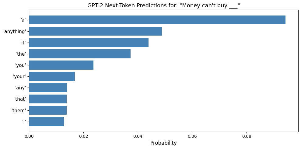
This is exactly what a language model does: given the context
'Money can't buy', it assigns a probability to every token in its
vocabulary (50,257 tokens) and picks the most likely continuation.